Purpose
Maximum likelihood estimation of the population parameters is performed with the button. The sequence of estimated parameters (
This algorithm produces the file pop_parameters.txt in the result folder, with all the estimated parameters: population parameters, variances (or standard deviations), correlations, error model parameters, etc. The estimation of the population parameters by groups defined by the continuous and categorical covariates used in the model is also given.
For example, in the theophylline_project, where one has a continuous covariate based on a transformation, the population parameters estimation file writes
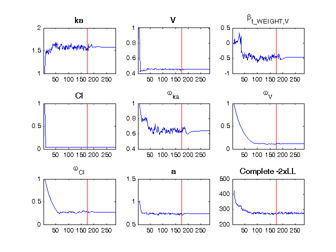
******************************************************************
* theophylline_project.mlxtran
* November 23, 2015 at 13:09:49
* Monolix version: 4.4.0
******************************************************************

Estimation of the population parameters

parameter
ka_pop : 1.57
V_pop : 0.454
beta_V_t_WEIGHT : -0.471
Cl_pop : 0.0399

omega_ka : 0.641
omega_V : 0.113
omega_Cl : 0.272

a : 0.735

Numerical covariates
t_WEIGHT = log(WEIGHT/70)
and the following figure is shown.
In another example, in the iov1_project, where we have both categorical covariates (SEX, TREAT, OCC, sTREAT) and IOV (the estimated parameters are called gamma), the population parameters estimation file writes
******************************************************************
*      iov1_project.mlxtran
*      November 24, 2015 at 08:44:55
*      Monolix version: 4.4.0
******************************************************************

Estimation of the population parameters

                   parameter
ka_pop           :     1.42
beta_ka_sTREATBA :    0.153
V_pop            :    0.469
beta_V_TREATB    :   -0.208
beta_V_sTREATBA  :   0.0415
beta_V_SEXM      :   0.0287
beta_V_OCC2      :  -0.0261
Cl_pop           :   0.0371
beta_Cl_SEXM     :  -0.0412
beta_Cl_OCC2     :   0.0188

omega_ka         :     0.26
omega_V          :   0.0957
omega_Cl         :    0.124

gamma_ka         :        0
gamma_V          :   0.0275
gamma_Cl         :    0.187

a                :    0.108
b                :    0.107
Main population parameter settings
Seed: The default value of the seed used for the random numbers generator is 123456. This seed can be randomly generated with the “generate” button. It is accessible in Menu/Settings/Seed.
Number of iterations: There are two stages in the population parameters estimation algorithm. Use K1 and K2 to define the number of iterations for each one. If auto is selected, then the algorithm will determine automatically if it can jump from one stage to the other or if it can finish the estimation process. In this case, the numbers 

")
Number of chains: When the data set is small, just a few of subjects for instance, replicating the data set can improve the precision of the estimation. The number of (Markov) chains specifies how many times the data set need to be replicated. You can specify this number yourself, or you can let Monolix to compute how many replicates are needed to ensure a minimum number of subjects. In this case, you should specify this minimum size and any time you change the data set, the number of chains will be updated according to the number of subjects present in the new data set. For instance, in the theophylline example there are only 12 subjects in the data set. Setting to 50 the minimum number of subjects, Monolix choose to use 5 Markov chains. It is accessible in Menu/Settings/Pop. parameters.
Simulated annealing: A Simulated Annealing version of SAEM is used to estimate the population parameters (the variances are constrained to decrease slowly during the first iterations of SAEM). It is accessible in Menu/Settings/Pop. parameters.
Very advance population parameters settings
In this paragraph, we define all the settings used for the population parameter estimation. However, we strongly encourage the user to get help from Lixoft’s support when considering using these parameters.
SAEM algorithm: Additionally, 
")


^{a_2}}")


MCMC: The default number of Markov chains is L = 1. 


Simulated Annealing: When Simulated Annealing is checked, the temperature decreases as 


What is and what is not SAEM? And the related implications.
The objective of this paragraph is to explain what is the SAEM, what the user can wait for and its limitation.
The SAEM algorithm is the stochastic approximation expectation-maximization algorithm. It has been shown to be extremely efficient for a wide variety of complex models: categorical data, count data, time-to-event data, mixture models, hidden Markov models, differential equation based models, censored data, … Furthermore, convergence of SAEM has been rigorously proved and the implementation in Monolix is efficient.
SAEM is an iterative algorithm: SAEM as implemented in Monolix has two phases. The goal of the first is to get to a neighborhood of the solution in only a few iterations. A simulated annealing version of SAEM accelerates this process when the initial value is far from the actual solution. The second phase consists of convergence to the located maximum with behavior that becomes increasingly deterministic, like a gradient algorithm.
SAEM is a stochastic algorithm: We cannot claim that SAEM always converges (i.e., with probability 1) to the global maximum of the likelihood. We can only say that it converges under quite general hypotheses to a maximum – global or perhaps local – of the likelihood. A large number of simulation studies have shown that SAEM converges with high probability to a “good” solution – it is hoped the global maximum – after a small number of iterations. Therefore, we encourage the user to use the convergence assessment tool to look at the sensitivity of the results w.r.t. the initial parameters
SAEM is a stochastic algorithm (2): The trajectory of the outputs of SAEM depends on the sequence of random numbers used by the algorithm. This sequence is entirely determined by the “seed.” In this way, two runs of SAEM using the same seed will produce exactly the same results. If different seeds are used, the trajectories will be different but convergence occurs to the same solution under quite general hypotheses. However, if the trajectories converge to different solutions, that does not mean that any of these results are “false”. It just means that the model is case sensitive to the seed or to the initial conditions.