Residuals | Monolix

Purpose

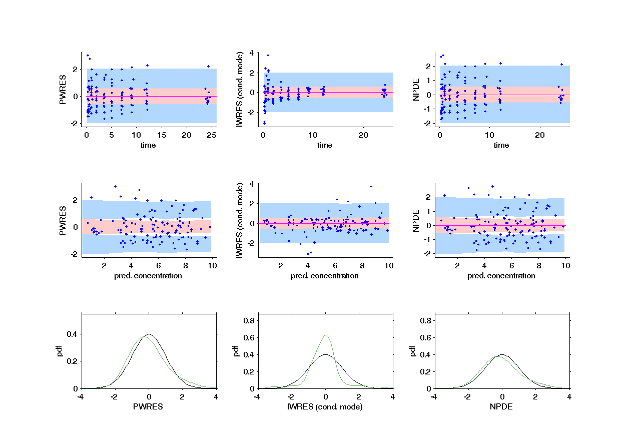
This graphic displays the PWRES (population weighted residuals), the IWRES (individual weighted residuals), and the NPDE (Normalized Prediction Distribution Errors) w.r.t. the time (on the top) and the prediction (bottom). The PWRES are computed using the population parameters and the IWRES are computed using the individual parameters. For discrete outputs, only NPDE and individual NPDE are used.

Population Weighted Residuals ( $\text{PWRES}_{ij}$ ) are defined as the normalized difference between the observations and their mean. Let $y_i = (y_{ij}, 1 \leq j \leq n_i)$ be the vector of observations for subject i. The mean of $y_i$ is the vector $\mathbb{E}(y_i)=(\mathbb{E}(f(t_{ij};\psi_i), 1 \leq j \leq n_i)\$ . Let $\text{V}_i$ be the $n_i \times n_i$ variance-covariance matrix of $y_i$ . Then, the ith vector of the population weighed residuals $\text{PWRES}_i=(\text{PWRES}_{ij}, 1\leq j \leq n_i)$ is defined by

$\text{PWRES}_i = \text{V}_i^{-1/2}(y_i-\mathbb{E}(y_i))$

$\mathbb{E}(y_i)$ and $V_i$ are not known in practice but can be estimated by Monte-Carlo simulation.

Individual weighted residuals ( $\text{IWRES}_{ij}$ ) are estimates of the standardized residual ( $\epsilon_{ij}$ ) based on individual predictions

$\text{IWRES}_{ij} = \dfrac{ y_{ij}-f(t_{ij};\hat{\psi}_i)}{g(t_{ij};\hat{\psi}_i)}$

If the residual errors are assumed to be correlated, the individual weighted residuals can be decorrelated by multiplying each individual vector $\text{IWRES}_i = (\text{IWRES}_{ij} ; 1\leq j\leq n_i)$ by $\hat{\text{R}}_i^{-1/2}$ , where $\hat{\text{R}}_i$ is the estimated correlation matrix of the vector of residuals $(\epsilon_{ij}; 1\leq j \leq n_i)$ .

Normalized prediction distribution errors ( $\text{NPDE}_{ij}$ ) are a nonparametric version of $\text{PWRES}_{ij}$ based on a rank statistic. For any (i,j), let $\text{F}_{ij} = \text{F}_{\text{PWRES}_{ij}}(\text{PWRES}_{ij})$ where $\text{F}_{\text{PWRES}_{ij}}$ is the cumulative distribution function (cdf) of $\text{PWRES}_{ij}$ . NPDEs are defined as an empirical estimation of $\Phi^{-1}(\text{F}_{ij})$ . In practice, one simulates a large number $K$ of simulated data set $y^{(k)}$ using the model, and estimate $\text{F}_{ij}$ as the fraction of simulated data below the original data, i.e:

$\hat{\text{F}}_{ij}=\frac{1}{K}\sum_{k=1}^K 1_{y_{ij}^{(k)}\leq y_{ij}^{\text{obs}}}$

By definition, the distribution of $\text{F}_{ij}$ is uniform on [0,1], we thus rather use $\Phi^{-1}(\text{F}_{ij})$ , which follows a standard normal distribution (with $\Phi$ the cdf of the standard normal distribution). NPDEs are defined as an empirical estimation of $\Phi^{-1}(\text{F}_{ij})$ , i.e $\text{NPDE}_{ij}=\Phi^{-1}(\hat{\text{F}}_{ij})$ .

For continuous outputs, this figure shows the empirical distributions of the weighted residuals and the NPDE together with the standard Gaussian pdf and qqplots to check if the residuals are Gaussian.

Example of graphic

In the following example, the parameters of a one compartmental model with first order absorption and linear elimination (on the theophylline data set) are estimated. One can see the PWRES, the IWRES and the NPDE w.r.t. the time (on the top), to the prediction (in the middle) and the comparison between the empirical and theoretical pdf of the PWRES, IWRES and NPDE are presented on the bottom. Notice, that in that example, the prediction intervals were added.

residuals

Settings

Residuals: The user can choose which residual will be displayed
- PWRES
- IWRES (using the individual parameter estimated using the conditional mode or the conditional mean)
- NPDE
Select Graphics: The user can define which graphics will be represented
- Scatter Plot (TIME): the representation w.r.t. the time
- Scatter Plot (Predictions): the representation w.r.t. the prediction
- Histogram: the pdf of the associated residual
- QQ-plot for the residuals.
Scatter Plot
- Observed data can be added
- BLQ data (and a possibility to add a different color) can be added if present
- Spline interpolation can be added
- Empirical percentiles for the 10%, 50% and 90% quantiles
- Theoretical percentiles for the 10%, 50% and 90% quantiles
- Prediction interval for the 10%, 50% and 90% quantiles
- Outliers (in dots or in area) to show the residuals that are out of the prediction interval
- By default, both displays are proposed with the individual parameters coming from the conditional mode estimation.
Residual Distribution
- Empirical pdf
- Theoretical pdf
- Histogram

By default, all the residuals and all the graphics are displayed.