Bayesian feature : on the use of priors on a fixed effect

When you select to define a prior distribution on a fixed effect, a new window will open to define its law as in the following

Bayesian

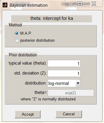
As for individual parameters, you can choose from some given distributions (normal, log-normal, logit-normal and probit-normal) or you can define your own as a transform T of a Gaussian distributed variable.
Assuming $\theta$ to be the chosen fixed effect with the transformation $\theta = T(Z)$ where $Z \sim {\cal N} (\mu_Z; \sigma^2_Z)$ is a Gaussian distributed variable. You must specify $m_{\theta}$ the typical value of $\theta$ ( $\mu_Z = T^{-1}(m_{\theta})$ and the variance or standard deviation of Z. By default, the current initial value will be used as typical value. Also, selecting a different typical value will set it automatically as initial value for the corresponding parameter. The user can also choose between two estimation methods: M.A.P. and posterior distribution.
Notice that Monolix can estimate the M.A.P only for

gaussian priors if the parameter is a covariate coefficient (a “ $\beta$ ”)
priors with same distribution than the corresponding individual parameter if $\theta$ is an intercept. It means that if V is set as log-normal distributed, then the M.A.P of $\theta$ ( $\theta =\textrm{intercept of V}$ ) can only be computed for log-normal priors on $\theta$ .