Introduction
Initial values are specified for the Fixed effects, for the Variances of the prandom effects and for the Residual error parameters. It is usually recommended to run SAEM with different initializations and to compare the results (this can be done via a convergence assessment, accessible through the “Assessment” button in the GUI).
Initialization of the “Fixed effects”
In this frame in the middle of the “Initialization” frame, the user can modify all the initial values of the fixed effects. There is at least on initial values by individual parameters. If no value is pre-defined (from a previously saved project for example), a default value at 1 is proposed. A right click on an initial value displays a list with three options.
- “Maximum likelihood estimation” (default): The parameter is estimated using maximum likelihood. In that case, the background remains white.
- “Fixed”: the parameter is kept to its initial value and so, it will not be estimated. In that case, the background is set to pink.
- “Bayesian estimation”: a pop-up windows opens to specify a prior distribution for this parameter. In that case, the background of the case is set to purple. To see more on the prior distribution, click here.
When an individual parameters depends on covariate, initial values for the dependency (named with 

In case of a continuous covariate, the covariate is added linearly to the transformed parameter, with a coefficient
In case of IOV, the same initialization is performed but in the IOV window when clicking on “IOV” on the right of the covariance model.
Initialization of the “Stand. dev. of the random effects”
In this frame in the middle of the “Initialization” frame, the user can modify all the initial values of the standard deviation of the random effects. The default value is set to 1. Each individual parameter has its initial value for the corresponding random effect. However, if the user specifies in the covariance model that a parameter has no variance (put 0 in the corresponding diagonal term of the covariance model), the corresponding standard deviation is set to 0 and the box is grayed to show the user that no modification can be done. A right click on an initial value displays a list with two options: “Maximum likelihood estimation” (default choice), and “Fixed”.
A button is added to offer the possibility to work with either the variance or the standard deviation. Notice that the transformations are done automatically by Monolix.
Initialization of the “Residual error parameters”
In this frame on the right of the “Initialization” frame, the user can modify all the initial values of the residual error parameters. There are as many lines as outputs of the model. The non-grayed values depend on the considered observation model. The default value depends on the parameter (1 for “a”, 0.3 for “b” and 1 for “c”). A right click on an initial value displays a list with two options: “Maximum likelihood estimation” (default choice), and “Fixed”.
How to initialize your parameters?
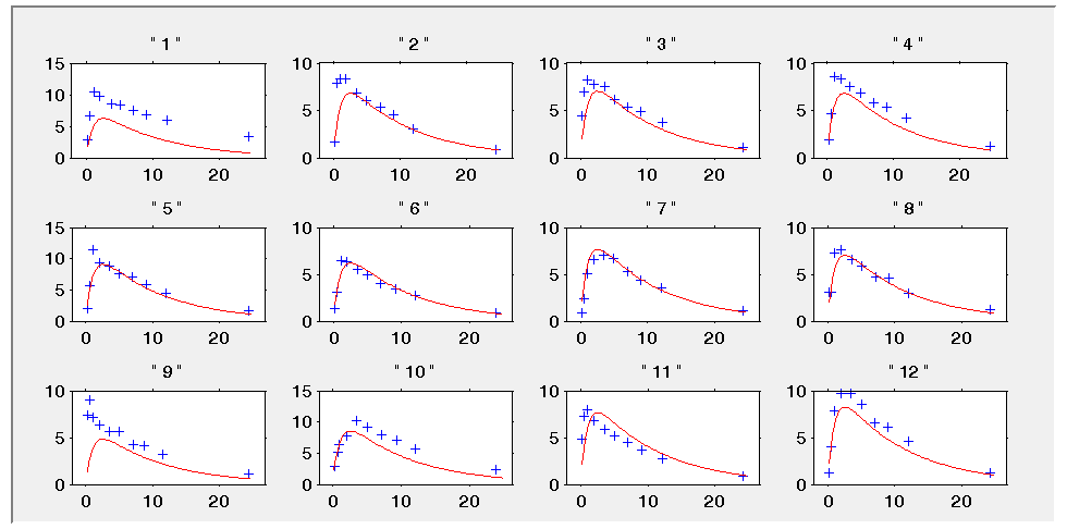
Check initial fixed effects
When clicking on the “Check the initial fixed effects” button, a pop-up window opens. The simulations obtained with the initial population fixed effects values are displayed for each individual together with the data points, in case of continuous observations. This feature is very useful to find some “good” initial values. Although Monolix is quite robust with respect to initial parameter values, good initial estimates speed up the estimation. You can change the values of the parameters with the buttons + and – and see how the agreement with the data change.
On the use of Mlxplore
Another convenient method is to use Mlxplore to have an initial guess. For that, you can export your model to Mlxplore (blue button next to the modle file in the Monolix GUI) and play with the initial values to see your model response. In the “Data” tab of the Mlxplore GUI, you can choose to overlay your data on top of the simulation. The main interest, compared to the “check the initial fixed effects” feature, is that you can also modify your structural model.
On the use of last estimates
If you have already estimated the population parameters for this project, then you can use the “Use the last estimates” button to use the previous estimates as initial values.