Complex parameter-covariate relationships and time-dependent covariates

Covariate-parameter relationships are usually defined via the Monolix GUI, leading for instance to exponential and power law relationships. However more complex parameter-covariate relationships such as Michaelis-Menten or Hill dependencies cannot the defined via the GUI because they cannot be put into the format where the (possibly transformed) covariate is added linearly on the transformed parameter. Similarly, when the covariate value is changing over time and thus not constant for each subject (or each occasion in each subject in case of occasions), the covariate cannot be added to the model via the GUI. In both cases, the effect of the covariate must be defined directly in the model file.

In the following, we will use as an example a Hill relationship between the clearance parameter Cl and the time-varying post-conception age (PCA) covariate, which is a typical way to scale clearance in paediatric pharmacokinetics:

$Cl_i = Cl_{pop} \frac{PCA^n}{PCA^n+A50^n} e^{\eta_i}$

where $Cl_i$ is the parameter value for individual i, $Cl_{pop}$ the typical clearance for an adult, $A50$ the PCA for the clearance to reach 50% mature, $n$ the shape parameter and $\eta_i$ the random effect for individual i.

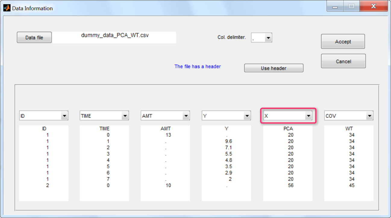
Step 1: To make the PCA covariate available as a variable is the model file, the first step is to tag it as a regressor column-type X when loading the data set (instead of using the COV and CAT column-types).

Step 2: In the model file, the PCA covariate is passed as input argument and designated as being a regressor. The clearance Cl, the hill shape parameter n, and the A50 are passed as usual input parameters:

[LONGITUDINAL]
input = {..., Cl, n, A50, PCA, ...}
PCA = {use=regressor}

If several regressors are used, be carefull that the regressors are matched by order with the data set columns tagged as X (not by name).

The relationship between the clearance Cl and the post-conception age PCA is defined in the EQUATION: block, before ClwithPCA is used (for instance in a simple (V,Cl) model):

EQUATION:
ClwithPCA = Cl * PCA^n / (PCA^n + A50^n)

Cc = pkmodel(Cl=ClwithPCA, V)

Note that the input parameter Cl includes the random effect ( $Cl = Cl_{pop} e^{\eta_i}$ ), such that only the covariate term must be added. Because the parameter including the covariate effect CLwithPCA is not a standard keyword for macros, one must write Cl=ClwithPCA.

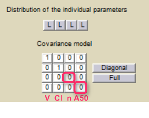
Step 3: The definition of the parameters in the GUI deserves special attention. Indeed the parameters n and A50 characterize the covariate effect and are the same for all individuals: their inter-individual variability must be removed by clicking on the corresponding diagonal elements of the variance-covariance matrix. On the opposite, the parameter Cl keeps its inter-individual variability, corresponding to the $e^{\eta_i}$ term.

Step 4: When covariates relationships are not defined via the GUI, the p-value corresponding to the Wald test is not automatically outputted. It is however possible to calculate it externally. Assuming that we would like to test if the shape parameter n is significantly different from 1:

$H_0:\quad \textrm{''}n=1\textrm{''} \quad \textrm{versus} \quad H_1:\quad \textrm{''}n \neq 1\textrm{''}$

Using the parameter estimate and the s.e outputted by Monolix, we can calculate the Wald statistic:

$W = \frac{\hat{n}-n_{ref}}{\textrm{s.e}(\hat{n})}$

with $\hat{n}$ the estimated value for parameter n, $n_{ref}$ the reference value for n (here 1) and $\textrm{s.e}(\hat{n})$ the standard error for the n estimate.

The test statistic W can then be compared to a standard normal distribution. Below we propose a simple R script to calculate the p-value:

 n_estimated = 1.32
 n_ref = 1
 se_n = 0.12
 
 W = abs(n_estimated - n_ref)/se_n
 
 pvalue = 2 * pnorm(W, mean = 0, sd = 1, lower.tail = FALSE)

Note that the factor 2 is added to do a two-sided test.