Objectives: learn how to define and use a PK model with multiple doses or assuming steady-state.
Projects: multidose_project, addl_project, ss1_project, ss2_project, ss3_project
Multiple doses
- multidose_project (data = ‘multidose_data.txt’ , model = ‘lib:bolus_1cpt_Vk.txt’)
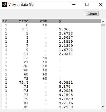
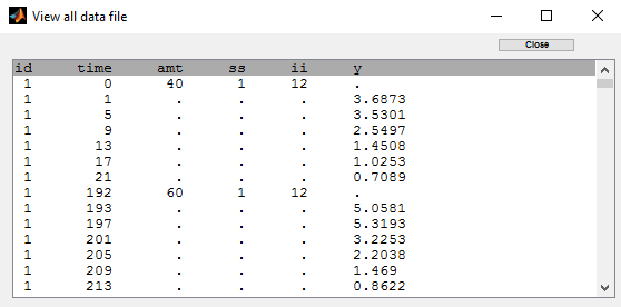
In this project, each patient receives several iv bolus injections. Each dose is represented by a row in the data file multidose_data.txt:
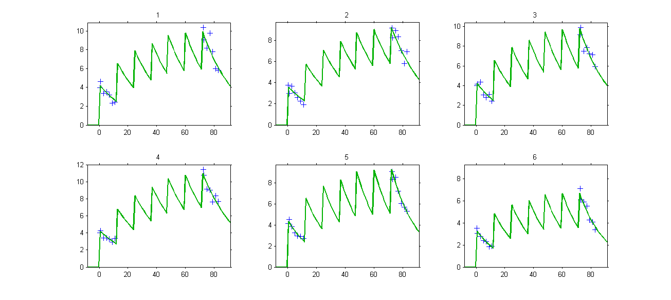
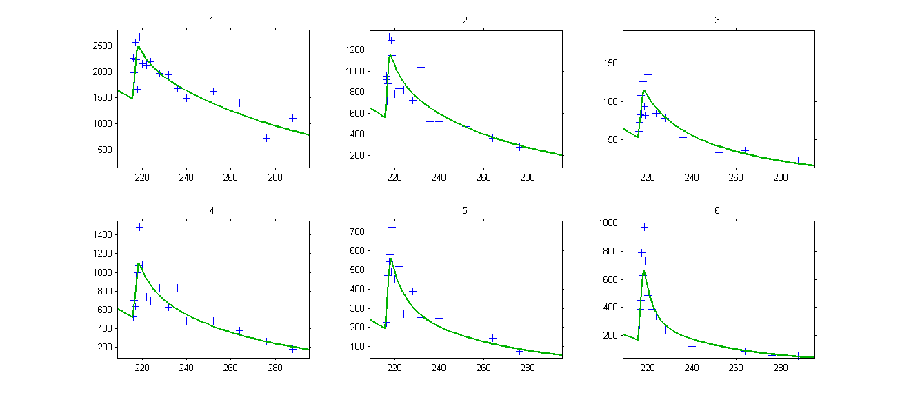
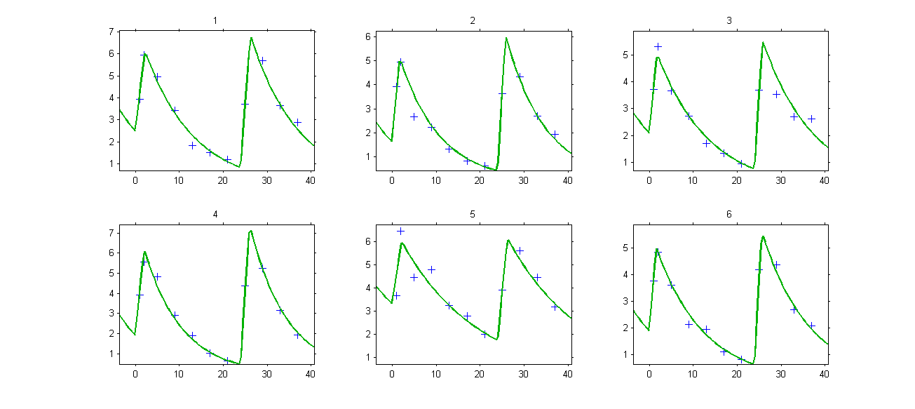
The PK model and the statistical model used in this project properly fit the observed data of each individual. Even if there is no observations between 12h and 72h, predicted concentrations computed on this time interval exhibit the multiple doses received by each patient:
VPCs, which is a diagnostic tool, are based on the design of the observations and therefore ignore” what may happen between 12h and 72h:
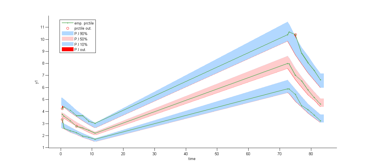
On the other hand, the prediction distribution, which is not a diagnostic tool, computes the distribution of the predicted concentration at any time point:
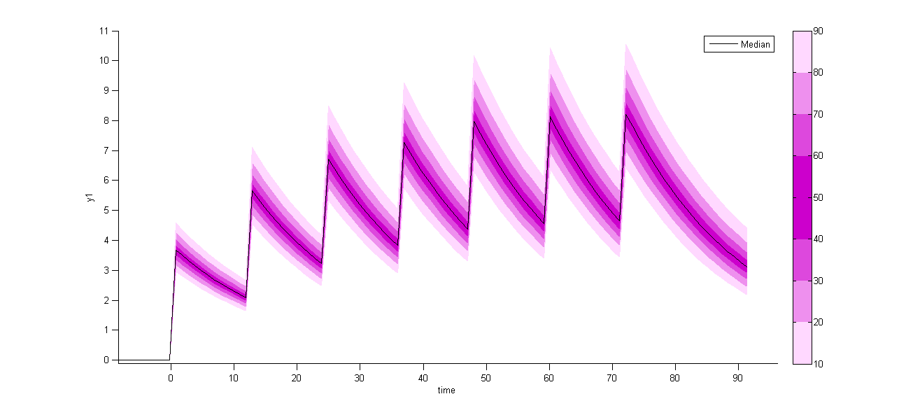
Additional doses (ADDL)
- addl_project (data = ‘addl_data.txt’ , model = ‘lib:bolus_1cpt_Vk.txt’)
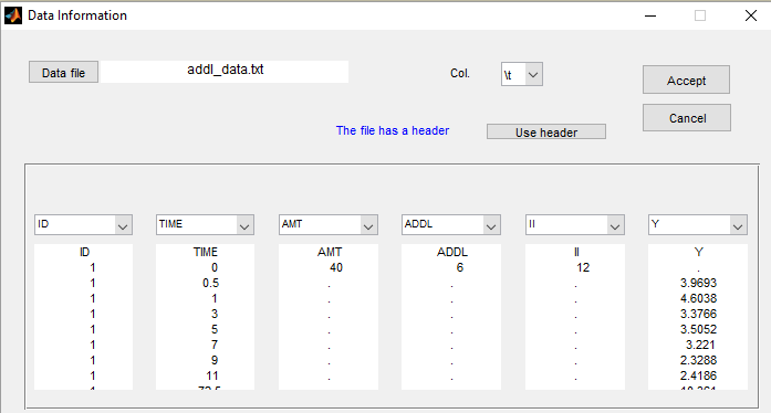
We can remark in the previous project, that, for each patient, the interval time between two successive doses is the same (12 hours for each patient) and the amount of drug which is administrated is always the same as well (40mg for each patient). We can take advantage of this design in order to simplify the data file by defining, for each patient, a unique amount (AMT), the number of additional doses which are administrated after the first one (ADDL) and the time interval between successive doses (II):
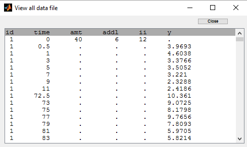
The keywords ADDL and II are automatically recognized by Monolix:
Remarks:
- Results obtained with this project, i.e. with this data file, are identical to the ones obtained with the previous project.
- It is possible to combine single doses (using ADDL=0) and repeated doses in a same data file.
Steady-state
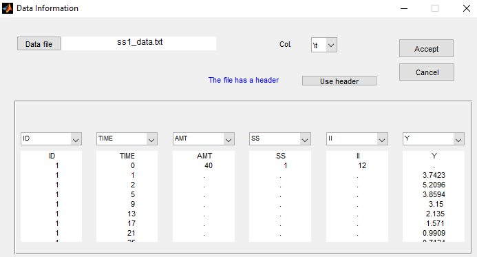
- ss1_project (data = ‘ss1_data.txt’ , model = ‘lib:oral0_1cpt_Tk0VCl.txt’)
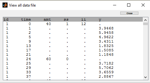
The dose orally administrated at time 0 to each patient is assumed to be a *steady-state dose* which means that a large” number of doses before time 0 have been administrated, with a constant amount and a constant interval dosing, such that steady-state, i.e. equilibrium, is reached at time 0. The data file ss1_data contains a column SS which indicates if the dose is a staedy-state dose or not and a column II for the inter-dose interval:
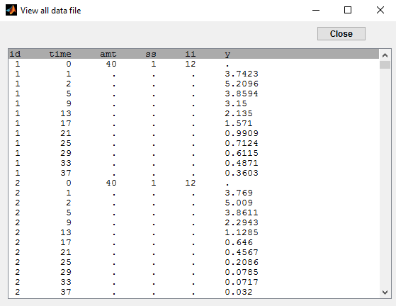
The keywords SS and II are automatically recognized by Monolix:
Click on Check the initial fixed effects and set the minimum value of the X-axis (min X) to display the predicted concentration between the last dose administrated at time 0:
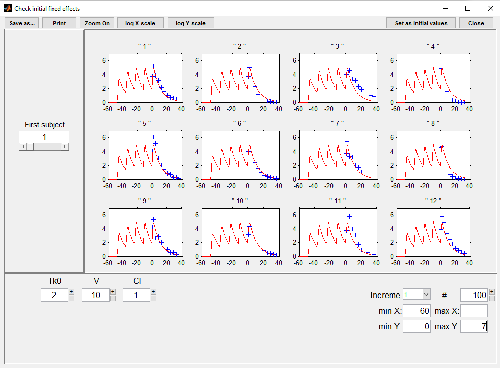
We see on this plot that Monolix adds 4 doses before the last dose to reach steady-state. Individual fits display the predicted concentrations computed with these additional doses:
- ss2_project (data = ‘ss2_data.txt’ , model = ‘lib:oral0_1cpt_Tk0VCl.txt’)
Steady-state and non steady-sates doses are combined in this project:
Individual fits display the predicted concentrations computed with this combination of doses:
- ss3_project (data = ‘ss3_data.txt’ , model = ‘lib:oral0_1cpt_Tk0VCl.txt’)
Two different steady-state doses are combined in this project:
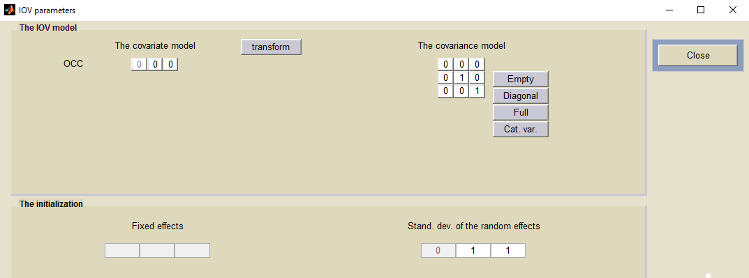
Monolix automatically creates occasions between successive steady-state doses in such situation. It is therefore possible to introduce inter-occasion variability (IOV) in the model: