Objectives: learn how to define and use a PK model for multiple routes of administration..
Projects: ivOral1_project, ivOral2_project
Combining iv and oral administrations – Example 1
- ivOral1_project (data = ‘ivOral1_data.txt’ , model = ‘ivOral1Macro_model.txt’)
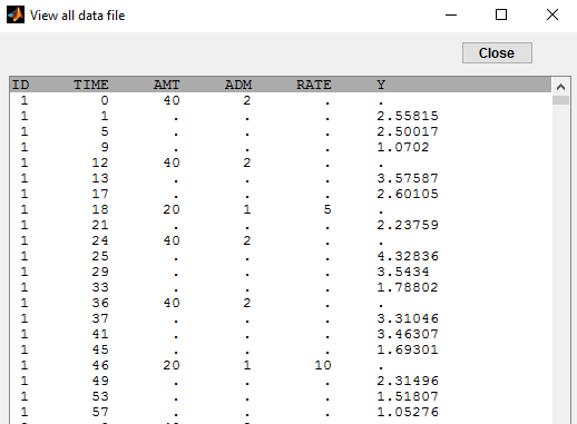
In this example, we combine oral and iv administrations of the same drug. The data file ivOral1_data.txt contains an additional column ADM which indicates the route of administration (1=oral, 2=iv):
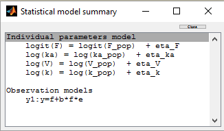
We assume here a one compartment model with first-order absorption process from the depot compartment (oral administration) and a linear elimination process from the central compartment. We further assume that only a fraction F (bioavailability) of the drug orally administered is absorbed. This model is implemented in ivOral1Macro_model.txt using PK macros:
[LONGITUDINAL]
input = {F, ka, V, k}
PK:
compartment(cmt=1, amount=Ac)
oral(type=1, cmt=1, ka, p=F)
iv(type=2, cmt=1)
elimination(cmt=1, k)
Cc = Ac/V
A logit-normal distribution is used for bioavability F that takes it values in (0,1):
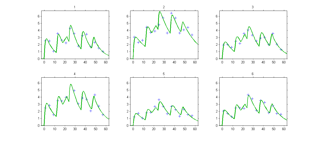
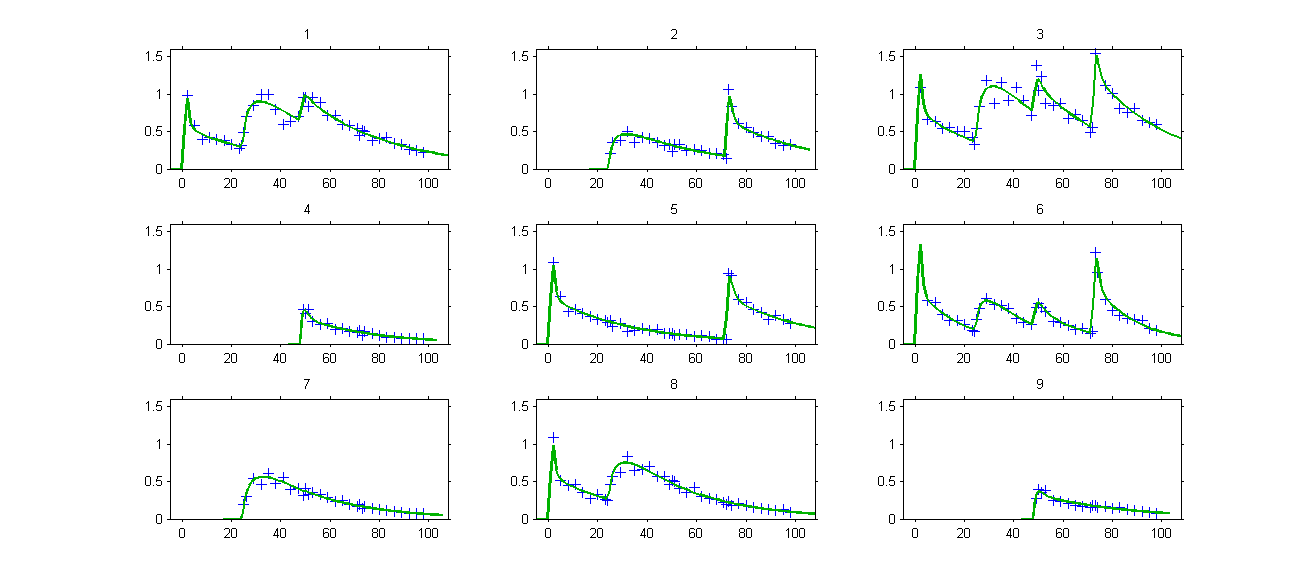
The model properly fits the data:
Remark: the same PK model could be implemented using ODEs instead of PK macros.
Let 

 & = - ka \, A_d(t) \\ \dot{A}_c(t) & = ka \, A_d(t) - k \, A_c(t) \end{aligned}")
The target compartment is the depot compartment (ivOral1ODE_model.txt using a system of ODEs:
[LONGITUDINAL]
input = {F, ka, V, k}
PK:
depot(type=1, target=Ad, p=F)
depot(type=2, target=Ac)
EQUATION:
ddt_Ad = -ka*Ad
ddt_Ac =  ka*Ad - k*Ac
Cc = Ac/V
Solving this ODEs system is less efficient than using the PK macros which uses the analytical solution of the linear system.
Combining iv and oral administrations – Example 2
- ivOral2_project (data = ‘ivOral2_data.txt’ , model = ‘ivOral2Macro_model.txt’)
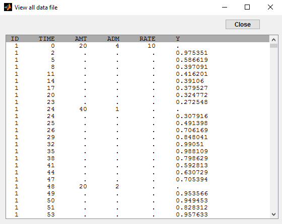
In this example (based on simulated PK data), we combine intraveinous injection with 3 different types of oral administrations of the same drug. The datafile ivOral2_data.txt contains column ADM which indicates the route of administration (1,2,3=oral, 4=iv):
We assume that one type of oral dose (adm=1) is absorbed into a latent compartment following a zero-order absorption process. the 2 oral doses (adm=2,3) are absorbed into the central compartment following first-order absorption processes with different rates. Bioavailabilities are supposed to be different for the 3 oral doses. There is linear transfer from the latent to the central compartment. A peripheral compartment is linked to the central compartment. The drug is eliminated by a linear process from the central compartment:
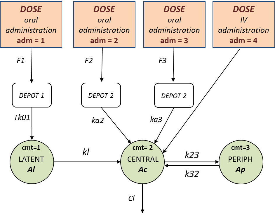
This model is implemented in ivOral2Macro_model.txt using PK macros:
[LONGITUDINAL]
input = {F1, F2, F3, Tk01, ka2, ka3, kl, k23, k32, V, Cl}
PK:
compartment(cmt=1, amount=Al)
compartment(cmt=2, amount=Ac)
peripheral(k23,k32)
oral(type=1, cmt=1, Tk0=Tk01, p=F1)
oral(type=2, cmt=2, ka=ka2,   p=F2)
oral(type=3, cmt=2, ka=ka3,   p=F3)
iv(type=4, cmt=2)
transfer(from=1, to=2, kt=kl)
elimination(cmt=2, k=Cl/V)
Cc = Ac/V
OUTPUT:
output = Cc
Here, logit-normal distributions are used for bioavabilities 


Remark: the number and type of doses vary from one patient to another one in this example.