- Joint model for continuous PK and categorical PD data
- Joint model for continuous PK and count PD data
- Joint model for continuous PK and time-to-event data
Objectives: learn how to implement a joint model for continuous and non continuous data.
Projects: warfarin_cat_project, PKcount_project, PKrtte_project
Joint model for continuous PK and categorical PD data
- warfarin_cat_project (data = ‘warfarin_cat_data.txt’, model = ‘PKcategorical1_model.txt’)
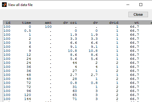
In this example, the original continuous PD data has been recoded as 1 (Low), 2 (Medium) and 3 (High).
More details about the data
International Normalized Ratio (INR) values are commonly used in clinical practice to target optimal warfarin therapy. Low INR values (<2) are associated with high blood clot risk and high ones (>3) with high risk of bleeding, so the targeted value of INR, corresponding to optimal therapy, is between 2 and 3.
Prothrombin complex activity is inversely proportional to the INR. We can therefore associate the three ordered categories for the INR to three ordered categories for PCA: Low PCA values if PCA is less than 33% (corresponding to INR>3), medium if PCA is between 33% and 50% (
The column dv contains both the PK and the new categorized PD measurements.
Instead of modeling the original continuous PD data, we can model the probabilities of each of these categories, which have direct clinical interpretations. The model is still a joint PKPD model since this probability distribution is expected to depend on exposure, i.e., the plasmatic concentration predicted by the PK model. We introduce an effect compartment to mimic the effect delay. Let }")
}")
} \leq 1 | \psi_i)\right) &= &\alpha_{i} + \beta_{i} Ce(t_{ij}^{(2)},\phi_i^{(1)}) \\ \text{logit} \left(\mathbb{P}(y_{ij}^{(2)} \leq 2 | \psi_i)\right) &=& \alpha_{i} + \gamma_{i} + \beta_{i}Ce(t_{ij}^{(2)},\phi_i^{(1)}) \\ \text{logit} \left(\mathbb{P}(y_{ij}^{(2)} \leq 3 | \psi_i)\right) &= & 1,\end{array}")
where })")


}")


If 
}=1")
},\phi_i^{(1)})")
[LONGITUDINAL]
input = {Tlag, ka, V, Cl, ke0, alpha, beta, gamma}
EQUATION:
{Cc,Ce}= pkmodel(Tlag,ka,V,Cl,ke0)
lp1 = alpha + beta*Ce
lp2 = lp1+ gamma         ; gamma >= 0
DEFINITION:
Level = {
  type=categorical
    categories={1,2,3}
    logit(P(Level<=1)) = lp1
    logit(P(Level<=2)) = lp2
}
OUTPUT:
output = {Cc, Level}
In this example, the residual error model for the PK data is defined in the Monolix GUI. We can equivalently use the model file PKcategorical2_model.txt where the the residual error model is defined in the model file:
[LONGITUDINAL]
input = {Tlag, ka, V, Cl, ke0, alpha, beta, gamma, a, b}
EQUATION:
{Cc,Ce}= pkmodel(Tlag,ka,V,Cl,ke0)
lp1 = alpha + beta*Ce
lp2 = lp1+ gamma         ; gamma >= 0
DEFINITION:
Concentration = {
  distribution=normal,
    prediction=Cc,
    errorModel=combined1(a,b)
}
Level = {
    type=categorical
    categories={1,2,3}
    logit(P(Level<=1)) = lp1
    logit(P(Level<=2)) = lp2
}
OUTPUT:
output = {Concentration, Level}
To use this model with the Monolix project, right click on the button Model file and select Change model. See Categorical data model for more details about categorical data models.
Joint model for continuous PK and count PD data
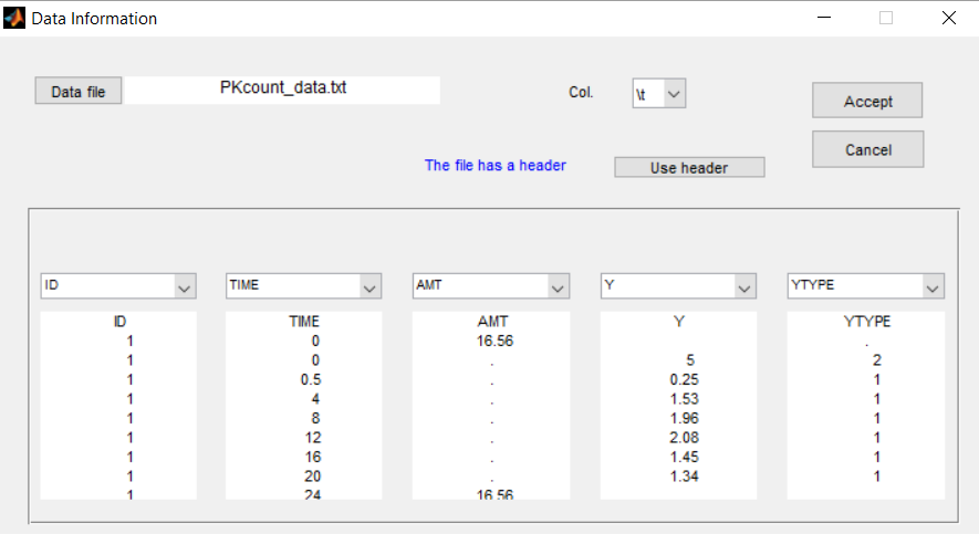
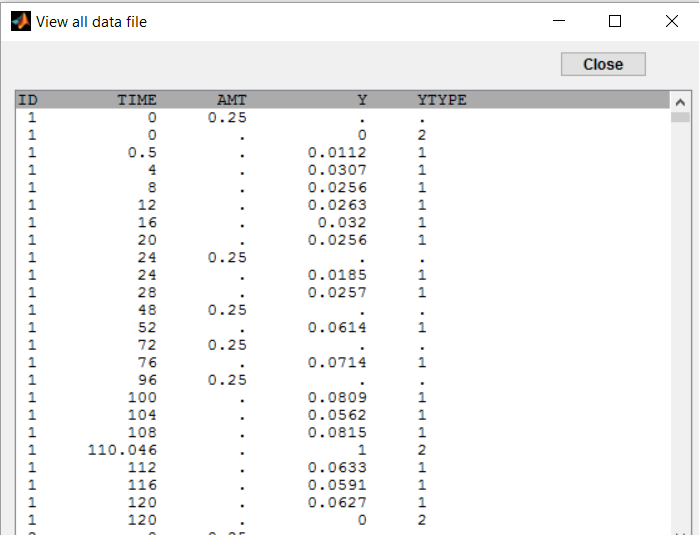
- PKcount_project (data = ‘PKcount_data.txt’, model = ‘PKcount1_model.txt’)
The data file used for this project is PKcount_data.txt where the PK and the count PD data are simulated data.
We use a Poisson distribution for the count data, assuming that the Poisson parameter is function of the predicted concentration. For any individual i, we have
 = \lambda_{0,i} \left( 1 - \frac{Cc_i(t)}{Cc_i(t) + IC50_i} \right)")
where ")
} = k)\right) = -\lambda_i(t_{ij}) + k\,\log(\lambda_i(t_{ij})) - \log(k!)")
The joint model is implemented in the model file PKcount1_model.txt
[LONGITUDINAL]
input = {ka, V, Cl, lambda0, IC50}
EQUATION:
Cc = pkmodel(ka,V,Cl)
lambda=lambda0*(1 - Cc/(IC50+Cc))
DEFINITION:
Seizure = { type = count,  log(P(Seizure=k)) = -lambda + k*log(lambda) - factln(k) }
OUTPUT:
output={Cc,Seizure}
Model file PKcount1_model.txt can be replaced by PKcount2_model.txt where the residual error model for the PK data is defined. See Count data model for more details about count data models.
Joint model for continuous PK and time-to-event data
- PKrtte_project (data = ‘PKrtte_data.txt’, model = ‘PKrtteWeibull1_model.txt’)
The data file used for this project is PKrtte_data.txt where the PK and the time-to-event data are simulated data.
We use a Weibull model for the events count data, assuming that the baseline is function of the predicted concentration. For any individual i, we define the hazard function as
 = \gamma_{i} \, Cc_i(t) \, t^{\beta-1}")
where
[LONGITUDINAL]
input  = {ka, V, Cl, gamma, beta}
EQUATION:
Cc = pkmodel(ka, V, Cl)
if t<0.1
  aux=0
else
  aux = gamma*Cc*(t^(beta-1))
end
DEFINITION:
Hemorrhaging  = {type=event, hazard=aux}
OUTPUT:
output = {Cc, Hemorrhaging}
Model file PKrtteWeibull1_model.txt can be replaced by PKrtteWeibull2_model.txt where the residual error model for the PK data is defined. See Time-to-event data model for more details about time-to-event data models.