- Introduction
- Fitting first a PK model to the PK data
- Simultaneous PKPD modeling using the PK and PD libraries
- Simultaneous PKPD modeling using a user defined model
- Sequential PKPD modelling
- Fitting a PKPD model to the PD data only
- Case studies
Objectives: learn how to implement a joint model for continuous PKPD data.
Projects: warfarinPK_project, warfarinPKPDlibrary_project, warfarinPKPDelibrary_project, warfarin_PKPDimmediate_project, warfarin_PKPDeffect_project, warfarin_PKPDturnover_project, warfarin_PKPDseq1_project, warfarin_PKPDseq2_project, warfarinPD_project
Introduction
A “joint model” describes two or more types of observation that typically depend on each other. A PKPD model is a “joint model” because the PD depends on the PK. Here we demonstrate how several observations can be modeled simultaneously. We also discuss the special case of sequential PK and PD modelling, using either the population PK parameters or the individual PK parameters as an input for the PD model.
Fitting first a PK model to the PK data
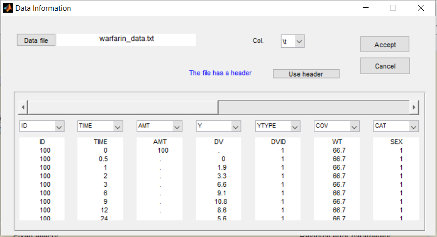
- warfarinPK_project (data = ‘warfarin_data.txt’, model = ‘lib:oral1_1cpt_TlagkaVCl.txt’)
The column DV of the data file contains both the PK and the PD measurements: the key-word Y is used by Monolix for this column. The column DVID is a flag defining the type of observation: DVID=1 for PK data and DVID=2 for PD data: the keyword YTYPE is then used for this column.
We will use the model oral1_1cpt_TlagkaVCl from the Monolix PK library
[LONGITUDINAL]
input = {Tlag, ka, V, Cl}
PK:
Cc = pkmodel(Tlag, ka, V, Cl)
OUTPUT:
output = Cc
Only the predicted concentration Cc is defined as an output of this model. Then, this prediction will be automatically associated to the outcome of type 1 (DVID=1) while the other observations (DVID=2) will be ignored.
Remark: any other ordered values could be used for YTYPE: the smallest one will always be associated to the first prediction defined in the model.
Simultaneous PKPD modeling using the PK and PD libraries
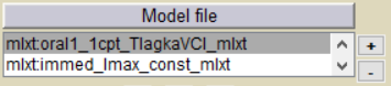
See project warfarinPKPDlibrary_project from demo folder 1.creating_and_using_models/libraries_of_models to see how to link the PK model to an immediate response model from the Monolix PD library for modelling simultaneously the PK and the PD warfarin data.
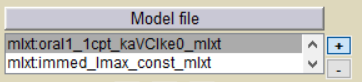
See project warfarinPKPDelibrary_project from demo folder 1.creating_and_using_models/libraries_of_models to see how to add an effect compartement by using the PKe and PDe Monolix libraries.
Simultaneous PKPD modeling using a user defined model
- warfarin_PKPDimmediate_project (data = ‘warfarin_data.txt’, model = ‘immediateResponse_model.txt’)
Is is also possible for the user to write his own PKPD model. The same PK model used previously and an immediate response model are defined in the model file immediateResponse_model.txt
[LONGITUDINAL]
input = {Tlag, ka, V, Cl, Imax, IC50, S0}
EQUATION:
Cc = pkmodel(Tlag, ka, V, Cl)
E = S0 * (1 - Imax*Cc/(Cc+IC50) )
OUTPUT:
output = {Cc, E}
Two predictions are now defined in the model: Cc for the PK (DVID=1) and E for the PD (DVID=2).
- warfarin_PKPDeffect_project (data = ‘warfarin_data.txt’, model = ‘effectCompartment_model.txt’)
An effect compartment is defined in the model file effectCompartment_model.txt
[LONGITUDINAL]
input = {Tlag, ka, V, Cl, ke0, Imax, IC50, S0}
EQUATION:
{Cc, Ce} = pkmodel(Tlag, ka, V, Cl, ke0)
E = S0 * (1 - Imax*Ce/(Ce+IC50) )
OUTPUT:
output = {Cc, E}
Ce is the concentration in the effect compartment
- warfarin_PKPDturnover_project (data = ‘warfarin_data.txt’, model = ‘turnover1_model.txt’)
An indirect response (turnover) model is defined in the model file turnover1_model.txt
[LONGITUDINAL]
input =  {Tlag, ka, V, Cl, Imax, IC50, Rin, kout}
EQUATION:
Cc = pkmodel(Tlag, ka, V, Cl)
E_0 = Rin/kout
ddt_E = Rin*(1-Imax*Cc/(Cc+IC50)) - kout*E
OUTPUT:
output = {Cc, E}
Several implementations of the same pkmodel are possible. For instance, the predicted concentration Cc is defined using equations in turnover2_model.txt instead of using the pkmodel function. The residual error models for the PK and PD measurements are both defined in turnover3_model.txt. Any of these two models can be used instead of turnover1_model.txt by right clicking on the Model file button and selecting Change model.
Sequential PKPD modelling
In the sequential approach, a PK model is developed and parameters estimated in the first step. For a given PD model, different strategies are then possible for the second step, i.e., for estimating the population PD parameters:
Using estimated population PK parameters
- warfarin_PKPDseq1_project (data = ‘warfarin_data.txt’, model = ‘turnover1_model.txt’)
Population PK parameters are set to their estimated values but individual PK parameters are not assumed to be known and sampled from their conditional distributions at each SAEM iteration. In Monolix, this simply means changing the status of the population PK parameter values so that they are no longer used as initial estimates for SAEM but considered fixed.
The joint PKPD model defined in turnover1_model.txt is again used with this project.
Using estimated individual PK parameters
- warfarin_PKPDseq2_project (data = ‘warfarinSeq_data.txt’, model = ‘turnoverSeq_model.txt’)
Individual PK parameters are set to their estimated values and used as constants in the PKPD model for the fitting the PD data. In this example, individual PK parameters ")
)")
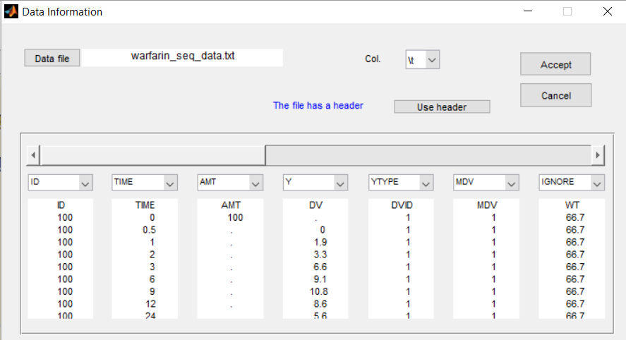
The estimated individual PK parameters are defined as regression variables, using the reserved keyword X. The covariates used for defining the distribution of the individual PK parameters are ignored.
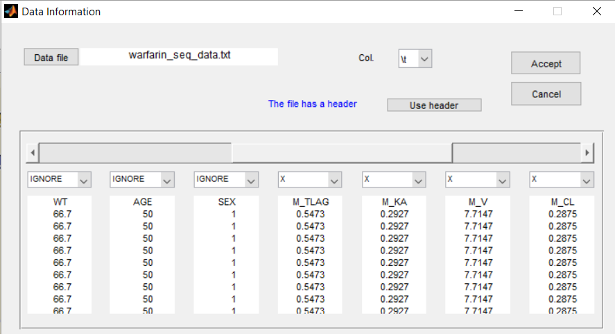
We use the same turnover model for the PD data. Here, the PK parameters are defined as regression variables (i.e. regressors).
[LONGITUDINAL]
input =  {Imax, IC50, Rin, kout, Tlag, ka, V, Cl}
Tlag  = {use = regressor}
ka    = {use = regressor}
V     = {use = regressor}
Cl    = {use = regressor}
EQUATION:
Cc = pkmodel(Tlag,ka,V,Cl)
E_0 = Rin/kout
ddt_E= Rin*(1-Imax*Cc/(Cc+IC50)) - kout*E
OUTPUT:
output = E
Fitting a PKPD model to the PD data only
- warfarinPD_project (data = ‘warfarinPD_data.txt’, model = ‘turnoverPD_model.txt’)
In this example, only PD data are available:
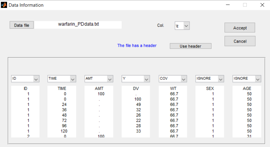
Nevertheless, a PKPD model – where only the effect is defined as a prediction – can be used for fitting this data:
[LONGITUDINAL]
input =  {Tlag, ka, V, Cl, Imax, IC50, Rin, kout}
EQUATION:
Cc = pkmodel(Tlag, ka, V, Cl)
E_0 = Rin/kout
ddt_E = Rin*(1-Imax*Cc/(Cc+IC50)) - kout*E
OUTPUT:
output = E
Case studies
- 8.case_studies/PKVK_project (data = ‘PKVK_data.txt’, model = ‘PKVK_model.txt’)
- 8.case_studies/hiv_project (data = ‘hiv_data.txt’, model = ‘hivLatent_model.txt’)