- Introduction
- Marginal distributions of the individual parameters
- Correlation structure of the random effects
Objectives: learn how to define the probability distribution and the correlation structure of the individual parameters.
Projects: warfarin_distribution1_project, warfarin_distribution2_project, warfarin_distribution3_project, warfarin_distribution4_project
Introduction
One way to extend the use of Gaussian distributions is to consider that some transformation of the parameters in which we are interested is Gaussian, i.e., assume the existence of a monotonic function 
")


 \sim {\cal N}(h(\bar{\psi}_i), \omega^2)")
where 


 \sim {\cal N}(h(\psi_{pop}), \omega^2)")
Transformation Monolix:
- Normal distribution:
The two mathematical representations for normal distributions are equivalent:
 ~~\Leftrightarrow~~ \psi_i = \bar{\psi}_i + \eta_i, ~~\text{where}~~\eta_i \sim {\cal N}(0,\omega^2).")
- Log-normal distribution:
A log-normally random variable takes positive values only. A log-normal distribution looks like a normal distribution for a small variance 
Remark: the two mathematical representations for log-normal distributions are equivalent:
 \sim {\cal N}(\log(\bar{\psi}_{i}), \omega^2) ~~\Leftrightarrow~~ \psi_i = \bar{\psi}_i e^{\eta_i}, ~~\text{where}~~\eta_i \sim {\cal N}(0,\omega^2).")
- Power-normal (or Box-Cox) distribution:
Here,  = \frac{\psi_i^\lambda -1}{\lambda}")

>0")


- Logit-normal distribution:
A random variable ")
 = \log \left(\frac{\psi_i}{1-\psi_i}\right) \ \sim \ \ {\cal N}( \text{logit}(\tilde{\psi}_i), \omega^2).")
- Probit-normal distribution:
A random variable 

")
 = \Phi^{-1}(\psi_i) \ \sim \ {\cal N}( \Phi^{-1}(\tilde{\psi}_i), \omega^2) .")
The probit-normal distribution with 

![[0,1]](http://s0.wp.com/latex.php?latex=%5B0%2C1%5D&bg=ffffff&fg=000&s=0 "[0,1]")
} = a + (b-a)\psi_{(0,1)} ,")
}")
Marginal distributions of the individual parameters
- warfarin_distribution1_project (data = ‘warfarin_data.txt’, model = ‘lib:oral1_1cpt_TlagkaVCl.txt’)
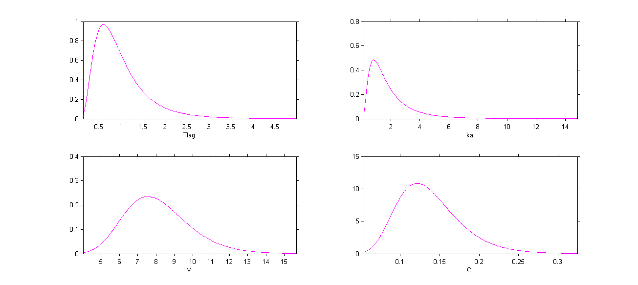
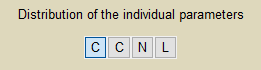
We use the warfarin PK example here. The four PK parameters Tlag, ka, V and Cl are log-normally distributed:
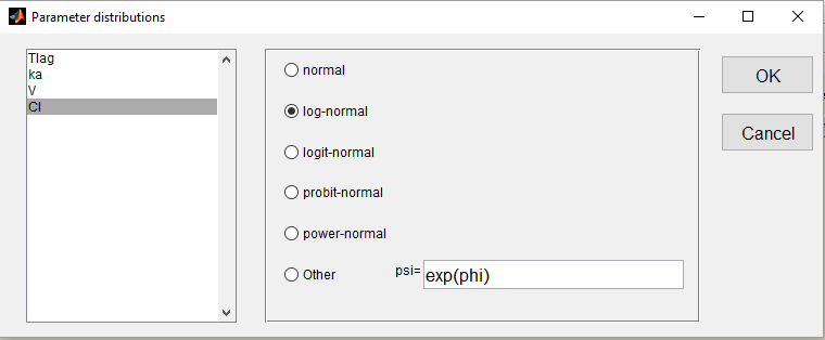
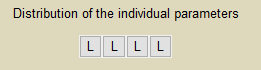
Letter L is then used for these four log-normal distributions in the main Monolix graphical user interface:
The distribution of the 4 PK parameters defined in the MonolixGUI is automatically translated into Mlxtran in the project file:
[INDIVIDUAL]
input = {Tlag_pop, omega_Tlag, ka_pop, omega_ka, V_pop, omega_V, Cl_pop, omega_Cl}
DEFINITION:
Tlag = {distribution=lognormal, typical=Tlag_pop, sd=omega_Tlag}
ka = {distribution=lognormal, typical=ka_pop, sd=omega_ka}
V = {distribution=lognormal, typical=V_pop, sd=omega_V}
Cl = {distribution=lognormal, typical=Cl_pop, sd=omega_Cl}
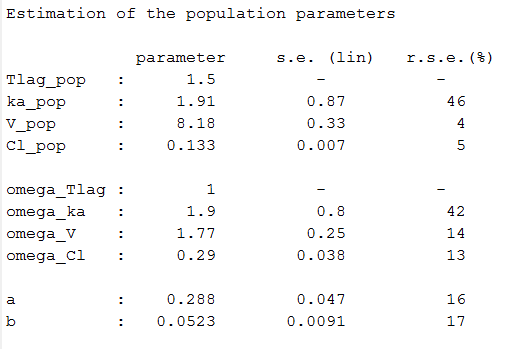
Estimated parameters are the parameters of the 4 log-normal distributions and the parameters of the residual error model:
Here, 

 \sim {\cal N}(\log(7.94) , 0.22^2)")

")
Remark: 
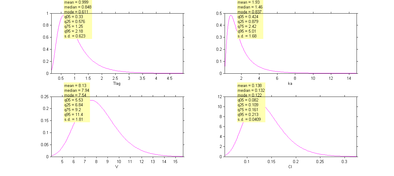
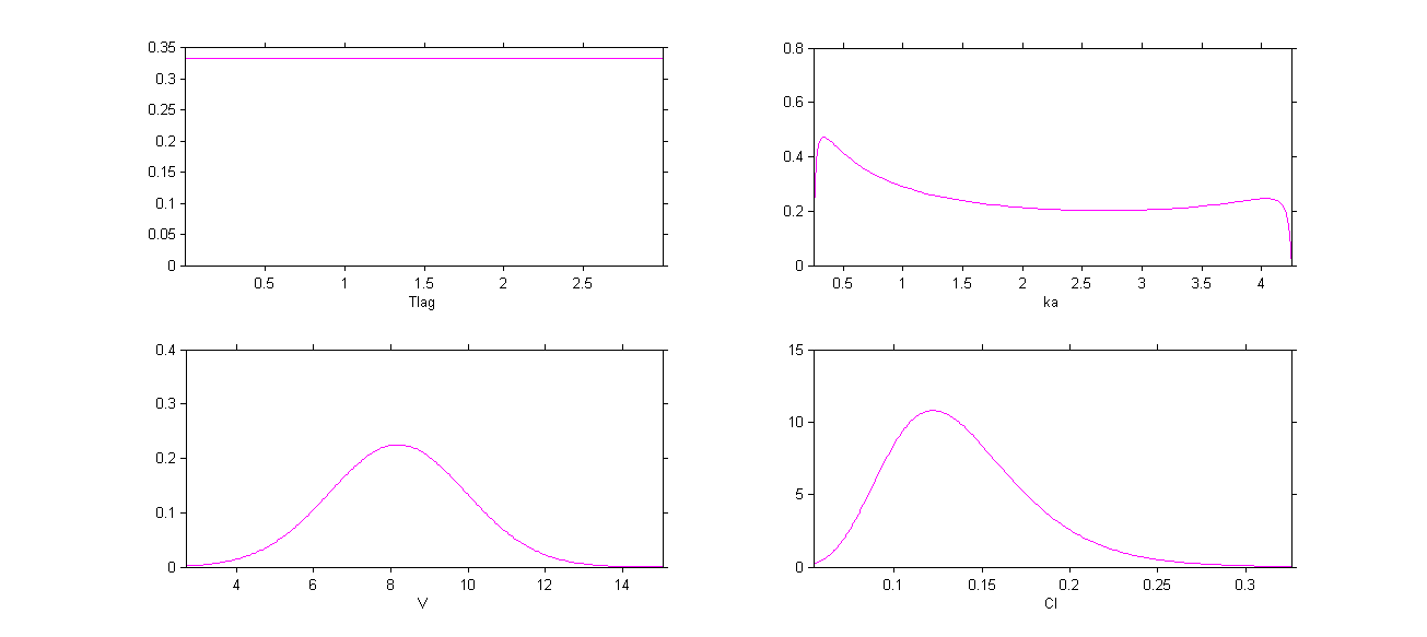
The four probability distribution functions are displayed Figure Parameter distributions:
Click on Settings and select the checkbox Informations to display a summary of these distributions:
Remark 1: 
Remark 2: here, standard deviations 


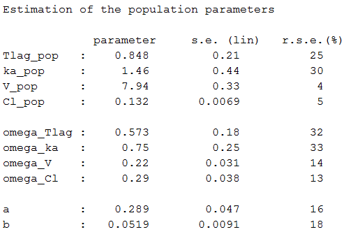
- warfarin_distribution2_project (data = ‘warfarin_data.txt’, model = ‘lib:oral1_1cpt_TlagkaVCl.txt’)
Other distributions for the PK parameters are used in this project:
- we use a uniform distribution on (0,3) for Tlag. This is equivalent to rescale a probit-normal distribution on (0,3)
and fix the population value 
- we use a logit-normal distribution rescaled on (0.25, 4.25) for ka:
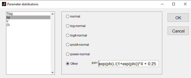
- a normal distribution for

- a log-normal distribution for

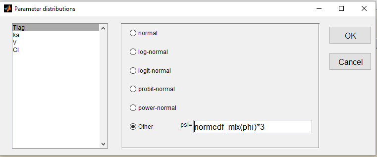
Distributions of Tlag and ka are therefore defined as Custom:
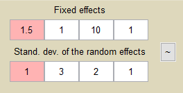
Estimated parameters are the parameters of the 4 transformed normal distributions and the parameters of the residual error model:
Here, 

![Tlag_i \sim Unif([0,3])](http://s0.wp.com/latex.php?latex=Tlag_i+%5Csim+Unif%28%5B0%2C3%5D%29&bg=ffffff&fg=000&s=0 "Tlag_i \sim Unif([0,3])")


 \sim {\cal N}(\textrm{logit}(\frac{1.91-0.25}{4}) , 1.9^2)")
The four probability distribution functions are displayed Figure Parameter distributions:
Remark 1: population values 

Remark 2: here, standard deviations 
Correlation structure of the random effects
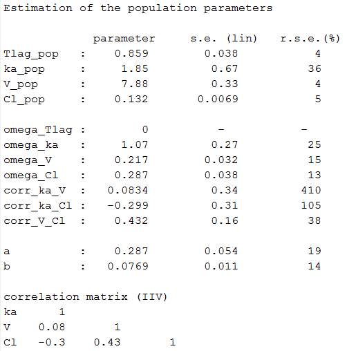
- warfarin_distribution3_project (data = ‘warfarin_data.txt’, model = ‘lib:oral1_1cpt_TlagkaVCl.txt’)
Correlation between the random effects can be introduced in the model. A block structure is used in this project, assuming linear correlations between 


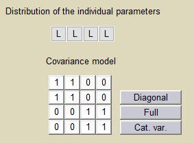
Estimated population parameters now include these 2 correlations:
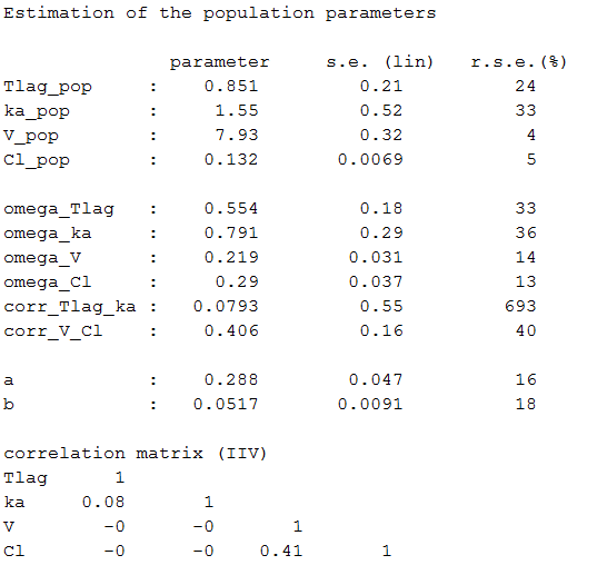
Remark: corr_Tlag_ka is not the correlation between the individual parameters 

- warfarin_distribution4_project (data = ‘warfarin_data.txt’, model = ‘lib:oral1_1cpt_TlagkaVCl.txt’)
In this example, 
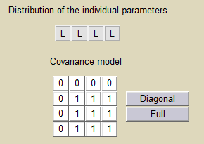
Estimated population parameters now include the 3 correlations between