- Introduction
- Defining the residual error model from the Monolix GUI
- Some basic residual error models
- Residual error models for bounded data
- Autocorrelated residuals
- Using different error models per group/study
Objectives: learn how to use the predefined residual error models.
Projects: warfarinPKlibrary_project, bandModel_project, autocorrelation_project, errorGroup_project
Introduction
For continuous data, we are going to consider scalar outcomes (
+ g(t_{ij},\psi_i,\xi_i)\varepsilon_{ij}")
for i from 1 to N, and j from 1 to 


")
")
")

 &= f(t_{ij},\psi_i) \\\textrm{sd}(y_{ij} | \psi_i) &= g(t_{ij},\psi_i,\xi)\end{aligned}")
The following error models are available in Monolix:
- constant :
and
- proportional :
and
- combined1 :
and
- combined2 :
and
- proportionalc :
and
- combined1c :
and
- combined2c :
and
 and
and 
 and
and 
 \varepsilon") and
and ")
 and
and  and
and ")
 \varepsilon") and
and ")
 and
and The assumption that the distribution of any observation
Model can be extended to include a transformation of the data:
=u(f(t_{ij},\psi_i))+ a\varepsilon_{ij}")
where u is a monotonic transformation (a strictly increasing or decreasing function). As we can see, both the data Monolix:
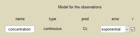
- exponential :
(assuming that
) and
. This is equivalent to assume that
.
 = \log(y)") (assuming that
(assuming that  ) and
) and )e^{ a\varepsilon_{ij}}") .
.- logit :
(assuming that
).
 = \textrm{logit}(y)=\log(y/(1-y))") (assuming that
(assuming that  ).
).- band(0,10) :
(assuming that
).
 = \textrm{logit}(y/10)=\log(y/(10-y))") (assuming that
(assuming that  ).
).- band(0,100) :
(assuming that
).
 = \textrm{logit}(y/100)=\log(y/(100-y))") (assuming that
(assuming that  ).
).Defining the residual error model from the Monolix GUI
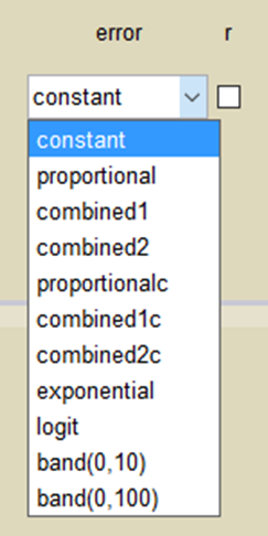
- A menu in the frame Data and model of the main GUI allows one to select the residual error model:
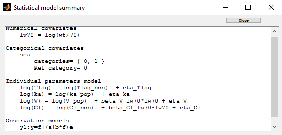
- a summary of the statistical model which includes the residual error model can be displayed:

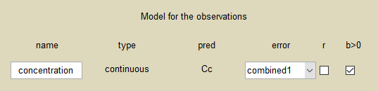
- when a combined 1 error model is used, we can force parameter b to be positive by ticking the box b>0:
- Autocorrelation of the residual errors is estimated when the checkbox r is ticked:
Some basic residual error models
- warfarinPKlibrary_project (data = ‘warfarin_data.txt’, model = ‘lib:oral1_1cpt_TlagkaVCl.txt’)
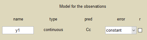
The residual error model used with this project for fitting the PK of warfarin is a constant error model
)+ a\varepsilon_{ij}")
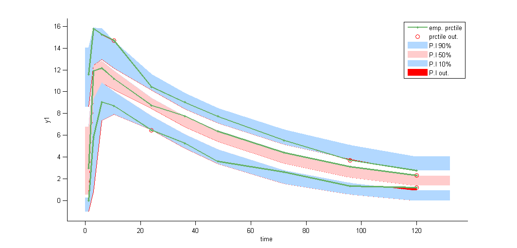
Several diagnostic plots can then be used for evaluating the error model. Here, the VPC’s suggests that a proportional component perhaps should be included in the error model:
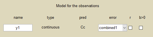
We can modify the residual error model and select, for instance, a combined1 error model directly from the menu in the GUI:
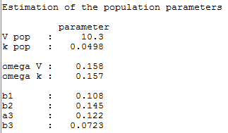
Estimated population parameters now include a and b

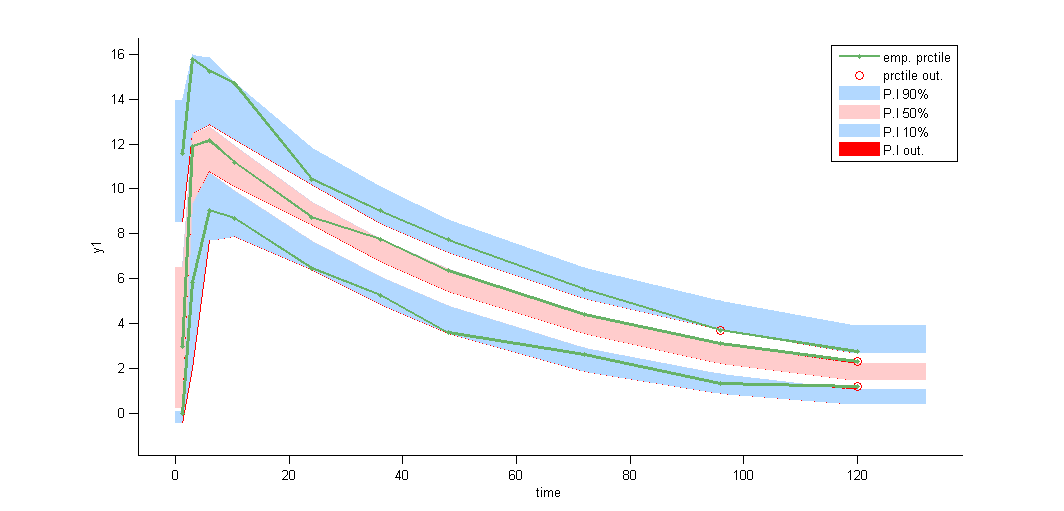
VPCs obtained with this error model do not show any mispecification
Remarks:
- When the residual error model is defined in the GUI, a bloc DEFINITION: is then automatically added to the project file in the section [LONGITUDINAL] of <MODEL> when the project is saved:
DEFINITION:
y1 = {distribution=normal, prediction=Cc, errorModel=combined(a,b)}
- the statistical summary includes the residual error model
Residual error models for bounded data
- bandModel_project (data = ‘bandModel_data.txt’, model = ‘lib:immed_Emax_null.txt’)
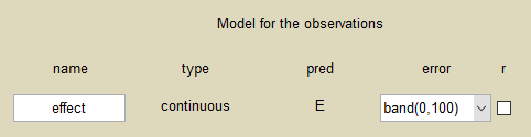
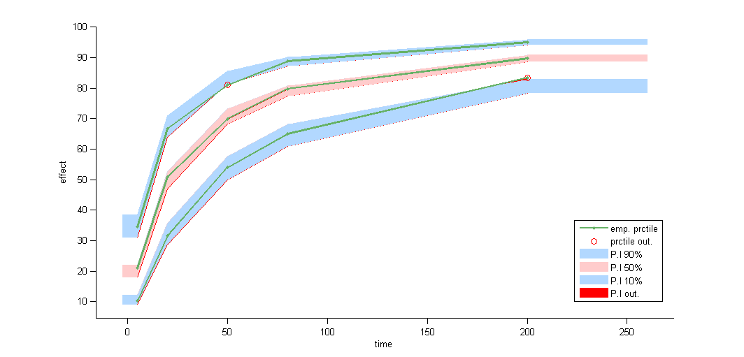
In this example, data are known to take their values between 0 and 100. We can use a band(0,100) error model if we want to take this constraint into account.
VPCs obtained with this error model do not show any mispecification
The statistical summary includes this residual error model:
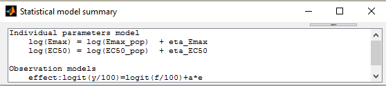
This residual error model is implemented in Mlxtran as follows:
DEFINITION:
effect = {distribution=logitnormal, min=0, max=100, prediction=E, errorModel=constant(a)}
Autocorrelated residuals
For any subject i, the residual errors ")
 = r_i^{(t_{i,j+1}-t_{ij})}")
where 


 &= {\rm corr}(\varepsilon_{ij},\varepsilon_{i,j+\tau}) \\&= r_i^{\tau} .\end{aligned}")
The residual errors are uncorrelated when 
- autocorrelation_project (data = ‘autocorrelation_data.txt’, model = ‘lib:infusion_1cpt_Vk.txt’)
Autocorrelation is estimated since the checkbox r is ticked in this project:
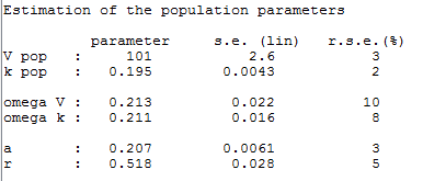
Estimated population parameters now include the autocorrelation r:
Remarks:
Monolixaccepts both regular and irregular time grids.- Rich data are required (i.e. a large number of time points per individual) for estimating properly the autocorrelation structure of the residual errors.
Using different error models per group/study
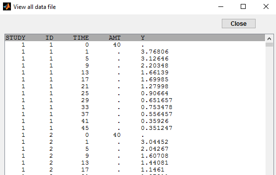
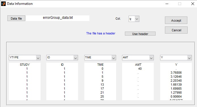
- errorGroup_project (data = ‘errorGroup_data.txt’, model = ‘errorGroup_model.txt’)
Data comes from 3 different studies in this example:
We want to use different error models for the 3 studies. A solution consists in defining the column STUDY with the reserved keyword YTYPE. It will be then possible to define one error model per outcome:
We use here the same PK model for the 3 studies:
[LONGITUDINAL]
input = {V, k}
PK:
Cc1 = pkmodel(V, k)
Cc2 = Cc1
Cc3 = Cc1
OUTPUT:
output = {Cc1, Cc2, Cc3}
Since 3 outputs are defined in the structural model, we can now define 3 error models in the GUI:
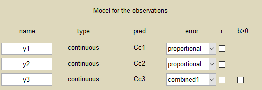
Different residual error parameters are estimated for the 3 studies. We can remark than, even if 2 proportional error models are used for the 2 first studies, different parameters