Longitudinal Model-Based Meta-Analysis (MBMA) with Monolix Suite

In this case study we demonstrate how to implement and analyze a longitudinal MBMA model with Monolix and Simulx.

Introduction
Background
- Canakinumab, a drug candidate for rheumatoid arthritis
- MBMA concepts
Data selection, extraction and visualization
Longitudinal mixed effect model description
Set up of the model in Monolix
Model development: Parameter estimation, model diagnosis, alternate model, covariate search, and final model
Simulations for decision support
- Comparison of canaki efficacy with drugs on the market
- Simulations of a Canaki versus Placebo clinical trial
Conclusion
Guidelines for implementing your own MBMA model

Introduction

Due to the high costs of drug development, it is crucial to determine as soon as possible during the drug development process if the new drug candidate has a reasonable chance of showing clinical benefit compared to the other compounds already on the market. To help the decision makers in go/no-go decisions, model-based meta-analysis (MBMA) has been proposed. MBMA consists in using published aggregate data from many studies to develop a model and support the decision process. Note that individual data are usually not available as only mean responses over entire treatment arms are reported in publications.

Because in an MBMA approach one considers studies instead of individuals, the formulation of the problem as a mixed effect model differs slightly from the typical PK/PD formulation. In this case study, we present how MBMA models can be implemented, analyzed and used for decision support in Monolix and Simulx.

As an example, we focus on longitudinal data of the clinical efficacy of drugs for rheumatoid arthritis (RA). The goal is to evaluate the efficacy of a drug in development (phase II) in comparison to two drugs already on the market. This case study is strongly inspired by the following publication:

Demin, I., Hamrén, B., Luttringer, O., Pillai, G., & Jung, T. (2012). Longitudinal model-based meta-analysis in rheumatoid arthritis: an application toward model-based drug development. Clinical Pharmacology and Therapeutics, 92(3), 352–9.

Canakinumab, a drug candidate for rheumatoid arthritis

Rheumatoid arthritis (RA) is a complex auto-immune disease, characterized by swollen and painful joints. It affects around 1% of the population and evolves slowly (the symptoms come up over months). Patients are usually first treated with traditional disease-modifying anti-rheumatic drugs, the most common being methotrexate (MTX). If the improvement is too limited, patients can be treated with biologic drugs in addition to the MTX treatment. Although biologic drugs have an improved efficacy, remission is not complete in all patients. To address this unmet clinical need, a new drug candidate, Canakinumab (abbreviated Canaki), has been developed at Novartis. After a successful proof-of-concept study, a 12-week, multicenter, randomized, double-blind, placebo-controlled, parallel-group, dose-finding phase IIB study with Canaki+MTX was conducted in patients with active RA despite stable treatment with MTX. In the study, Canaki+MTX was shown to be superior to MTX alone.

We would like to compare the expected efficacy of Canaki with the efficacy of two drugs already on the market, Adalimumab (abbreviated Adali) and Abatacept (abbreviated Abata). Several studies involving Adali and Abata have been published in the past (see list below). A typical endpoint in those studies is the ACR20, i.e the percentage of patients achieving 20% improvement. We focus in particular on longitudinal ACR20 data, measured at several time points after initiation of the treatment, and we would like to use a mixed effect model to describe this data.

MBMA concepts

The formulation of longitudinal mixed effect models for study-level data differs from longitudinal mixed effect models for individual-level data. As detailed in

Ahn, J. E., & French, J. L. (2010). Longitudinal aggregate data model-based meta-analysis with NONMEM: Approaches to handling within treatment arm correlation. Journal of Pharmacokinetics and Pharmacodynamics, 37(2), 179–201.

to obtain the study-level model equations, one can write a non-linear mixed effect model for each individual (including inter-individual variability) and derive the study-level model by taking the mean response in each treatment group, i.e the average of the individual responses. In the simplistic case of linear models, the study-level model can be rewritten such that a between-study variability (BSV), a between-treatment arm variability (BTAV) and a residual error appear. Importantly, in this formulation, the residual error and the between treatment arm variability are weighted by $\sqrt{N_{ik}}$ with $N_{ik}$the number of individuals in treatment arm k of study i. If the model is not linear, a study-level model cannot be easily derived from the individual-level model. Nevertheless, one usually makes the approximation that the study-level model can also be described using between-study variability, between-treatment arm variability and a residual error term.

This result can be understood in the following way: when considering studies which represent aggregated data, the between-study variability represents the fact that the inclusion criteria vary from study to study, thus leading to patient groups with slightly different mean characteristics from study to study. This aspect is independent of the number of individuals recruited. On the opposite, the between-treatment arm variability represents the fact that when the recruited patients are split in two or more arms, the characteristics of the arms will not be perfectly the same, because there is a finite number of individuals in each arm. The larger the arms are, the smaller the difference between the mean characteristics of the arms is, because one averages over a larger number. This is why the between-treatment arm variability is weighted by $\sqrt{N_{ik}}$. For the residual error, the reasoning is the same: as the individual-level residual error is averaged over a larger number of individuals, the study-level residual error decreases.

The study-level model can thus be written in a way similar to the individual-level model, except that we consider between-study variability and between-treatment arm variability instead of inter-individual variability and inter-occasion variability. And in addition, the residual error and the between treatment arm variability are weighted by $\sqrt{N_{ik}}$.

Before proposing a model for rheumatoid arthritis, let us first have a closer look at the data.

Data selection, extraction and visualization

Data selection

To compare Canaki to Adali and Abata, we have searched for published studies involving these two drugs. Reusing the literature search presented in Demin et al., we have selected only studies with inclusion criteria similar to the Canaki study, in particular: approved dosing regimens, and patients having an inadequate response to MTX. Compared to the Demin et al. paper, we have included two additional studies published later on. In all selected studies, the compared treatments are MTX+placebo and MTX+biologic drug.

The full list of used publications is:

Data extraction

Using an online data digitizer application, we have extracted the longitudinal ACR20 data of the 9 selected publications. The information is recorded in a data file, together with additional information about the studies. The in house individual Canaki data from the phase II trial is averaged over the treatments arms to be comparable to the literature aggregate data. Below is a screenshot of the data file, and a description of the columns.

excel_screenshot

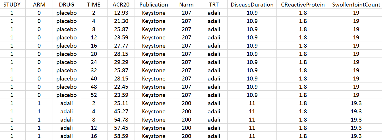
STUDY: index of the study/publication. (Equivalent to the ID column)
ARM: 0 for placebo arm (i.e MTX+placebo treatment), and 1 for biologic drug arm (MTX+biologic drug)
DRUG: name of the drug administrated in the arm (placebo, adali, abata or canaki)
TIME: time since beginning of the treatment, in weeks
ACR20: percentage of persons on the study having an at least 20% improvement of their symptoms
Publication: first author of the publication from which the data has been extracted
Narm: number of individuals in the arm
TRT: treatment studied in the study
DiseaseDuration: mean disease duration (in years) in the arm at the beginning of the study
CReactiveProtein: mean C-reactive protein level (in mg/dL)
SwollenJointCount: mean number of swollen joints

Data visualization

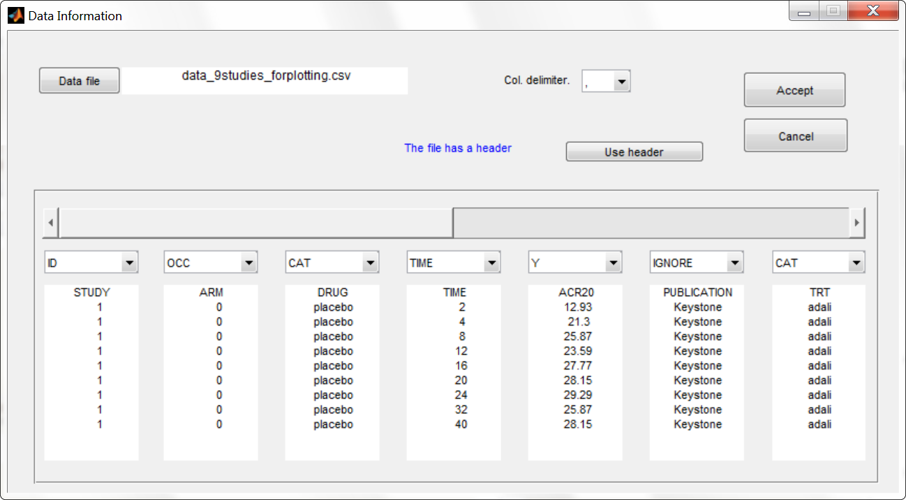
To gain a better overview of this data set, we first plot it. Because the MonolixSuite data visualization application, Datxplore, does not yet support occasions (needed to display the different arms of a study), we instead use the data plotting feature of Monolix. We load the data set in Monolix and assign the columns in the following way:

load_data_for_plot

We then click on the “plot the data” button next to the data loading frame, to see the data as a spaghetti plot. To better distinguish the treatments and arms, we go to “stratify” and choose to split by TRT and color by DRUG. We can in addition change the titles, labels and axes limits in “Axes > Settings”. In the following figure, arms with biologic drug treatment appear in color (abata in blue, adali in red, canaki in green), while placebo arms appear in black. Note that even in the “placebo” arms the ACR20 improves over time, due to the MTX treatment. In addition, we clearly see that the treatment MTX+biologic drug has a better (but not complete) efficacy compared to MTX+placebo. For Canaki, which is the in house drug in development, only one study is available, the phase II trial.

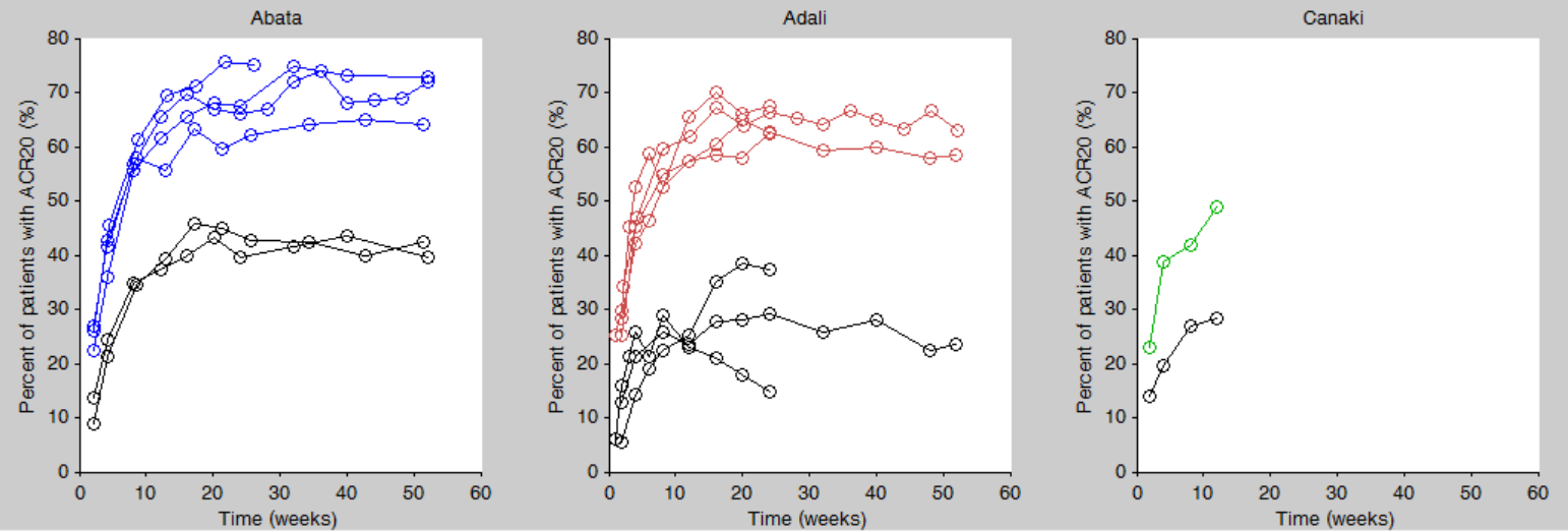
Given this data, does Canaki has a chance to be more effective than Adali and Abata? To answer this question, we develop a longitudinal mixed effect model.

Longitudinal mixed effect model description

Given the shape of the ACR20 over time, we propose an Emax structural model:

$$f(t)= \textrm{Emax}\frac{t}{t+\textrm{T50}}$$

Remember that the ACR20 is a fraction of responders, it is thus in the range 0-1 (or 0-100 if considering the corresponding percentage). In order to keep the model observations also in the range 0-1, we use a logit transformation for the observations $y_{ijk}$:

$$\textrm{logit}(y_{ijk})=\textrm{logit}(f(t_j,\textrm{Emax}_{ik},\textrm{T50}_{ik}))+\epsilon_{ijk}$$

with i the index over studies, j the index over time, and k the index over the treatment arms. $\epsilon_{ijk}$ is the residual error, it is distributed according to:

$$\epsilon_{ijk}\sim \mathcal{N}\left( 0,\frac{\sigma^2}{N_{ik}}\right)$$

with $N_{ik}$ the number of individuals in treatment arm k of study i. Because our data is quite scarce and our interest is mainly on the Emax (efficacy), we choose to consider between-study variability (BSV) and between treatment arm variability (BTAV) for Emax only. For Emax parameter distribution, we select a logit distribution to keep its values between 0 and 1. We thus have:

$$\textrm{logit}(\textrm{Emax}_{ik})=\textrm{logit}(\textrm{Emaxpop}_{d})+\eta^{(0)}_{\textrm{E},i}+\eta^{(1)}_{\textrm{E},ik}$$

$\eta^{(0)}_{\textrm{E},i}$ represents the BSV and $\eta^{(1)}_{\textrm{E},ik}$ represents the BTAV.

For T50, we select a log-normal distribution and no random-effects:

$$\textrm{log}(\textrm{T50}_{ik})=\textrm{log}(\textrm{T50pop}_{d})$$

with Emaxpop_d and T50pop_d the typical population parameters, that depend on the administrated drug d. The BSV (index (0)) and BTAV (index (1)) terms for Emax have the following distributions:

$$\eta^{(0)}_{\textrm{E},i}\sim\mathcal{N}\left( 0,\omega_E^2\right) \quad \eta^{(1)}_{\textrm{E},ik}\sim\mathcal{N}\left( 0,\frac{\gamma_E^2}{N_{ik}}\right)$$

In the next section, we describe how to implement this model in Monolix.

Set up of the model in Monolix

For the error model

In Monolix, it is only possible to choose the error model among a pre-defined list. This does not allow to have a residual error model weighted by the square root of the number of individuals. We will thus transform both the ACR20 observations of the data set and the model prediction in the following way, and use a constant error model. Indeed we can rewrite:

$$\begin{array}{ccl}\textrm{logit}(y_{ijk})=\textrm{logit}(f(t_j,\textrm{Emax}_{ik},\textrm{T50}_{ik}))+\epsilon_{ijk} & \Longleftrightarrow & \textrm{logit}(y_{ijk})=\textrm{logit}(f(t_j,\textrm{Emax}_{ik},\textrm{T50}_{ik}))+\frac{\tilde{\epsilon}_{ijk}}{\sqrt{N_{ik}}} \ & \Longleftrightarrow & \sqrt{N_{ik}} \times \textrm{logit}(y_{ijk})=\sqrt{N_{ik}} \times \textrm{logit}(f(t_j,\textrm{Emax}_{ik},\textrm{T50}_{ik}))+\tilde{\epsilon}_{ijk} \ &\Longleftrightarrow& \textrm{transY}_{ijk}=\textrm{transf}(t_j,\textrm{Emax}_{ik},\textrm{T50}_{ik}))+\tilde{\epsilon}_{ijk} \end{array} $$

with

$\tilde{\epsilon}_{ijk}$ a constant (unweighted) residual error term,
$\textrm{transY}_{ijk}=\sqrt{N_{ik}} \times \textrm{logit}(y_{ijk})$ the transformed data,
$\textrm{transf}(t_j,\textrm{Emax}_{ik},\textrm{T50}_{ik}))=\sqrt{N_{ik}} \times \textrm{logit}(f(t_j,\textrm{Emax}_{ik},\textrm{T50}_{ik}))$ the transformed model prediction.

This data transformation is added to the data set, in the column transY. At this stage, we can load the data set into Monolix. We assign the columns as shown above, except that we now use the column transY as Y. STUDY is tagged as ID, ARM as OCC, DRUG as CAT, Narm as regressor X and DiseaseDuration, CReactiveProtein and SwollenJointCount as continuous covariates COV.

To match the observation transformation in the data set, we will have in the Mlxtran model file:

ACR20 = ...
pred = logit(ACR20)*sqrt(Narm)
OUTPUT:
output = pred

In order to be available in the model, the data set column Narm must be tagged as regressor (type X), and passed as argument in the input list:

[LONGITUDINAL]
input = {..., Narm}
Narm = {use=regressor}

In our example the number of individuals per arm (Narm) is constant over time. In case of dropouts or non uniform trials, Narm may vary over time. This will be taken into account in Monolix as, by definition, regressors can change over time.

For the parameter distribution

Similarly to the error model, it is not possible to weight the BTAV directly via the Monolix GUI. As an alternative, we can define separately the fixed effect (EmaxFE), the BSV random effect (etaBSVEmax) and the BTAV random effect (etaBTAVEmax) in the GUI and reconstruct the parameter value within the model file. Because we have defined Narm as a regressor, we can use it to weight the BTAV terms. We also need to be careful about adding the random effects on the normally distributed transformed parameters. Here is the syntax:

[LONGITUDINAL]
input = {EmaxFE, T50, etaBSVEmax, etaBTAVEmax, Narm}
Narm = {use=regressor}

EQUATION:
; transform the Emax fixed effect (EmaxFE) to tEmax (normally distributed) 
tEmax = logit(EmaxFE)

; adding the random effects (RE) due to between-study variability and 
; between arm variability, on the transformed parameters 
tEmaxRE = tEmax + etaBSVEmax + etaBTAVEmax/sqrt(Narm)

; transforming back to have EmaxRE with logit distribution (values between 0 and 1)
EmaxRE = 1 / (1+ exp(-tEmaxRE) )

; defining the effect
ACR20 = EmaxRE * (t / (T50 + t))

; adding a saturation to avoid taking logit(0) (undefined) when t=0
ACR20sat = max(ACR20, 0.01)

; transforming the effect ACR20 in the same way as the data
pred = logit(ACR20sat)*sqrt(Narm)

OUTPUT:
output = pred

In addition to the steps already explained, we add a saturation ACR20sat=max(ACR20,0.01) to avoid having ACR20=0 when t=0, which would result in pred=logit(0) (which is undefined).

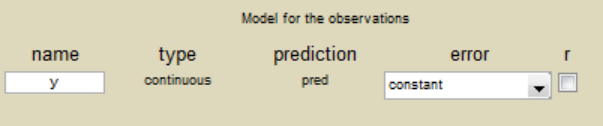
After having compiled and accepted the model in the “Model file” window, we continue the model set up via the GUI. For the residual error model, we choose “constant” from the list, according to the data transformation done.

focus_error_model
For the parameter distributions, we choose a logit distribution for EmaxFE, log-normal for T50, and a normal distribution for the random effects etaBSVEmax, and etaBTAVEmax. Because with this model formulation EmaxFE represents only the fixed effects, we need to disable the random effects for this parameter by clicking on the corresponding diagonal term of the variance-covariance matrix. This sets its variance to 0. We also disable the random effects for T50:

var-covar_NEW

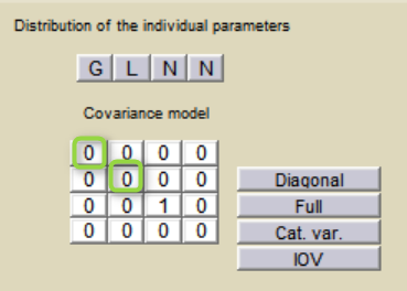
For etaBSVEmax, its distribution is $ \mathcal{N}(0,\omega^2) $ , we thus need to enforce its mean to be zero. This is done by fixing its fixed effect to 0 using a right click on the fixed effect initial value.

inival_NEW

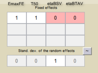
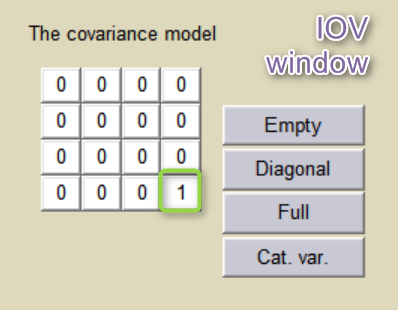
etaBTAVEmax is equivalent to inter-occasion variability, we thus disable its inter-subject (inter-study) variability (i.e enforce zero variance in the variance-covariance matrix of the main window), fix its fixed effect to 0 and we go to the IOV window (click on IOV button) to set the corresponding diagonal elements of the variance-covariance matrix at the IOV level to 1.

IOV_window_NEW

For the covariates

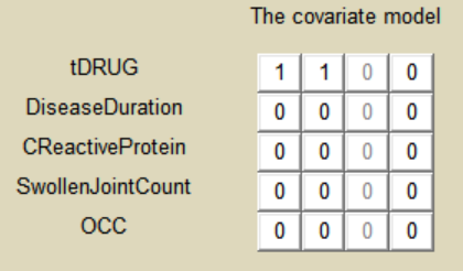
As a final step, we need to add DRUG as a covariate on EmaxFE and T50, in order to estimate one EmaxFE and one T50 value for each treatment (placebo, adali, abata, and canaki). Because the DRUG column is constant over an arm (<=> occasion) but not over a study (<=> ID), it appears in the IOV window and can be added there as categorical covariate on EmaxFE and T50. Before adding the DRUG column as covariate, we go to the “transform” window and set placebo as reference category. The new covariate is called tDRUG. The other possible covariates will be investigated later on.

cov_NEW

Summary view

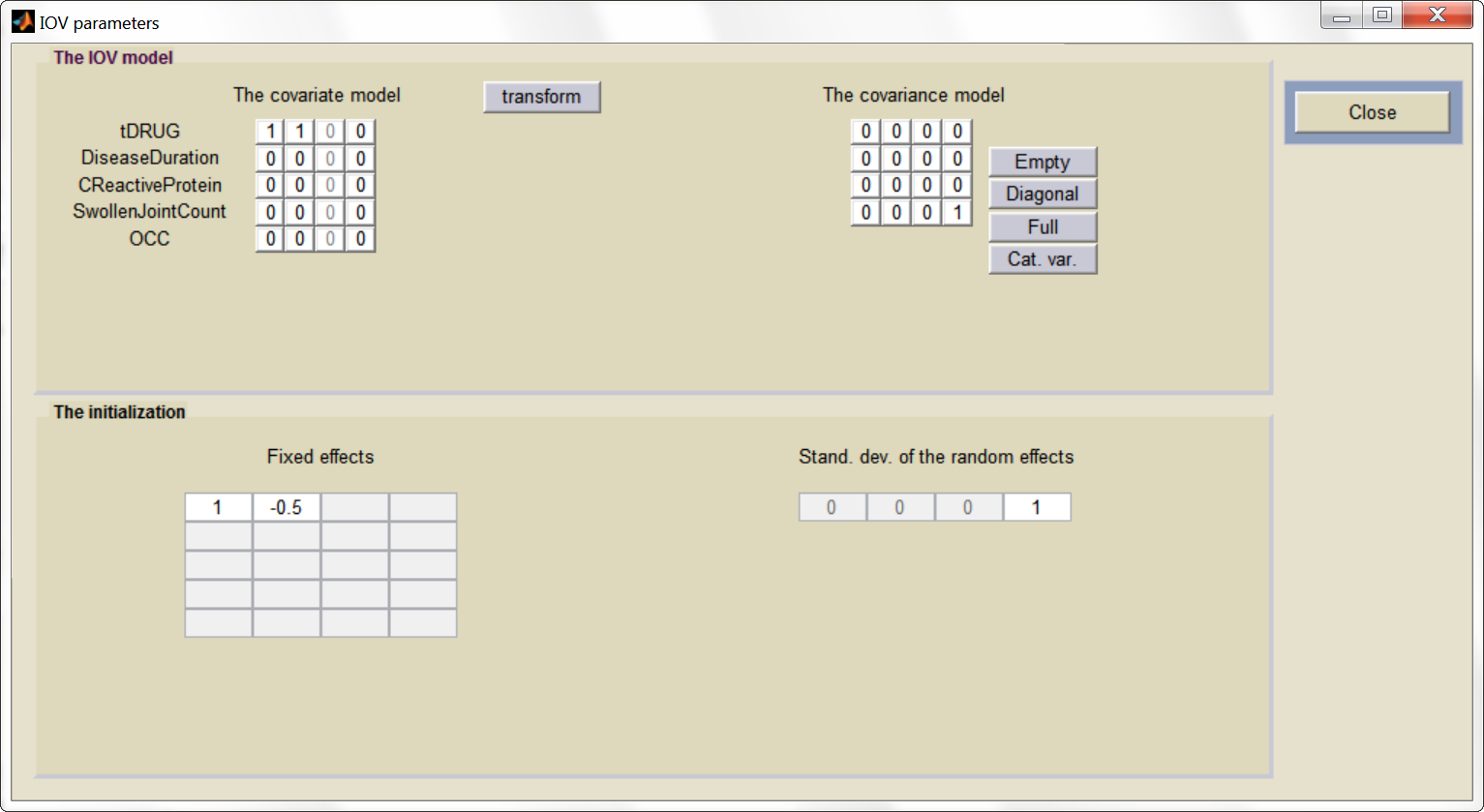
After this model set up, the main Monolix window is:

main_NEW

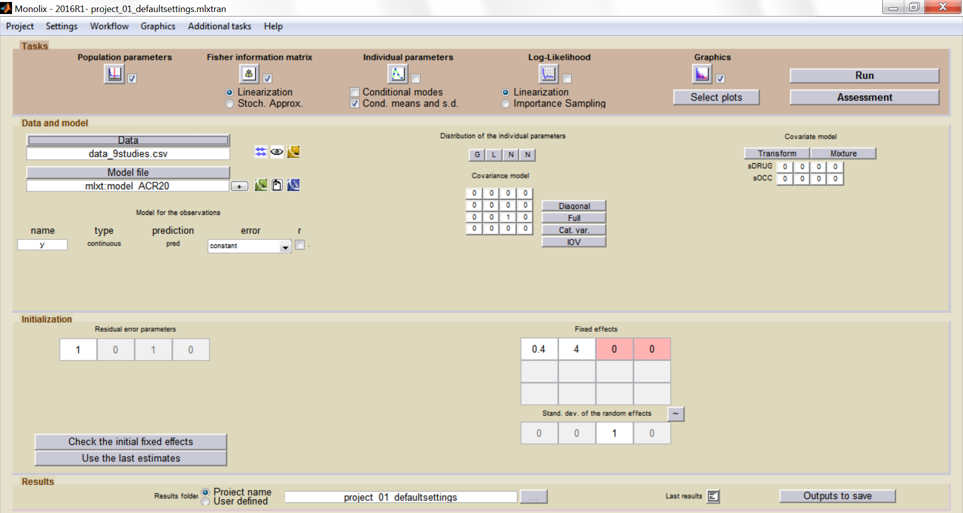
And the IOV window:

IOV_window_summary_NEW

Model development

Parameter estimation

Finding initial values

Before starting the parameter estimation, we first try to find reasonable initial values. In the “Check the initial fixed effects” window, we can adjust the EmaxFE and T50 initial parameter values by looking at the agreement between the population prediction (red line) and the data (blue crosses). We choose for instance EmaxFE=0.4 and T50=4.

checkini_NEW

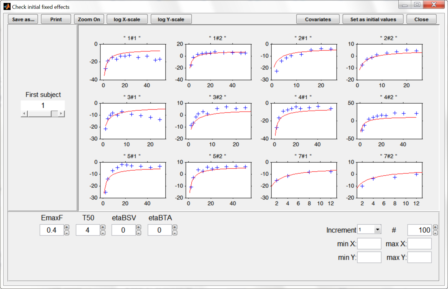
To let the initial value for the beta parameters (that characterize the values of EmaxFE and T50 in the case of treatment compared to the placebo case) appear one needs to click on the “covariates” button at the top of the window. The EmaxFE value for the drugs needs to be higher than for placebo, so we choose beta_EmaxFE_tDRUG=1. For beta_T50_tDRUG we choose -0.5 with the help of the “Check the initial fixed effects” plots.

Choosing the settings

We then launch the parameter estimation task. After around 110 iterations, the SAEM exploratory phase switches to the second phase, due to the automatic stopping criteria. The convergence looks rather good.

conv1_NEW

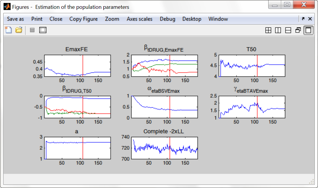
To assess the convergence, we can run the parameter estimation from different initial values and with a different random number sequence. To do so, we click on the “assessment” button and select “all”. 5 estimations run will be done using automatically drawn initial values. In the main window, the following tasks should be ticked: population and fisher information (to be able to compare the obtained estimates) via stochastic approximation for instance. The individual parameters, log-likelihood and graphics can be unticked to increase the speed.

assess1_NEW

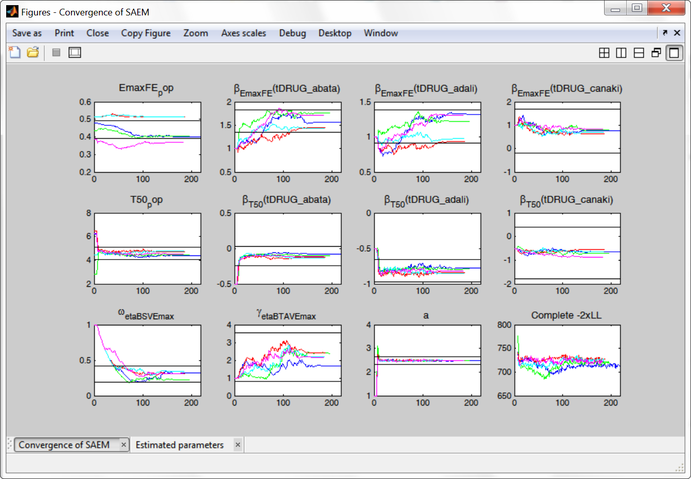
The colored lines show the parameter estimates trajectories, while the black lines show the standard deviation. We see that the parameters converge within the same standard error, except EmaxFE. Parameters without variability, such as EmaxFE, may be harder to estimate. Indeed, parameters with and without variability are not estimated in the same way. The SAEM algorithm requires to draw parameter values from their marginal distribution, which exists only for parameters with variability.

Several methods can be used to estimate the parameters without variability. By default, these parameters are optimized using the Nelder-Mead simplex algorithm (Matlab’s fminsearch method). As the performance of this method seems insufficient in our case, we will try another method. In “Settings > Pop. parameters > Advanced settings”, 4 options are available in the “zero-variability” section:

No variability (default): optimization via Nelder-Mead simplex algorithm (Matlab’s fminsearch method)
Add decreasing variability: an artificial variability is added for these parameters, allowing estimation via SAEM. The variability is progressively forced to zero, such that at the end of the estimation proces, the parameter has no variability.
Variability in the first stage: during the first phase, an artificial variability is added and progressively forced to zero. In the second phase, the Nelder-Mead simplex algorithm is used.
Mixed method: alternates between SAEM with an artifical variability and Nelder-Mead simplex algorithm

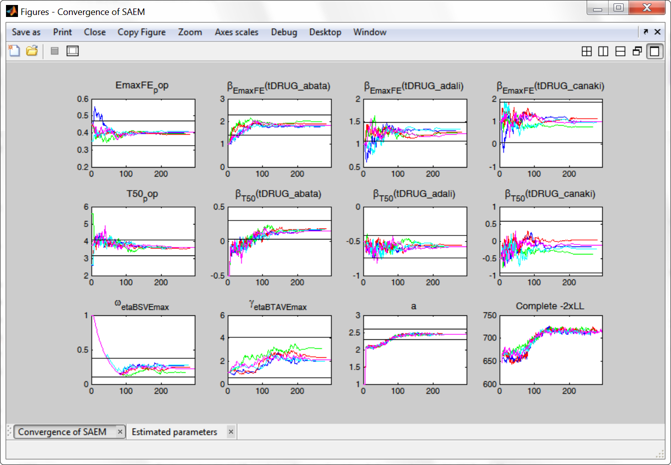
We choose the “variability in the first stage” method (the other methods give similar results), and launch the convergence assessment again. This time the convergence is satisfactory.

assess2_NEW

Results

We can either directly look as the estimated values in the *_rep folders that have been generated during the convergence assessment, or redo the parameter estimation and the estimation of the Fisher information matrix (via linearization for instance) to get the standard errors.

The estimated values are the following:

esti_NEW

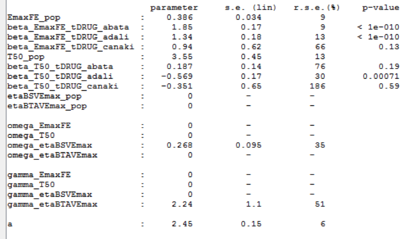
As indicated by the p-value (calculated via a Wald test), the Emax values for Abata and Adali are significantly different from the Emax for placebo. On the opposite, given the data, the Emax value for Canaki is not significantly different from placebo. Note that when analyzing the richer individual data for Canaki, the efficacy of Canaki had been found significantly better than that of placebo (Alten, R. et al. (2011). Efficacy and safety of the human anti-IL-1β monoclonal antibody canakinumab in rheumatoid arthritis: results of a 12-week, Phase II, dose-finding study. BMC Musculoskeletal Disorders, 12(1), 153.). The T50 values are similar for all compounds except Adali.

The between study variability of Emax is around 27%. The between treatment arm variability is gamma_etaBTAVEmax=2.24. In the model, the BTAV gets divided by the square root of the number of individuals per arm. If we consider a typical number of individual per arm of 200, the between treatment arm variability is around 16%.

Model diagnosis

We next estimate the study parameters (i.e individual parameters via mode task) and generate the graphics: no model mis-specification can be detected in the individual fits, observations versus predictions, residuals, and other graphics:

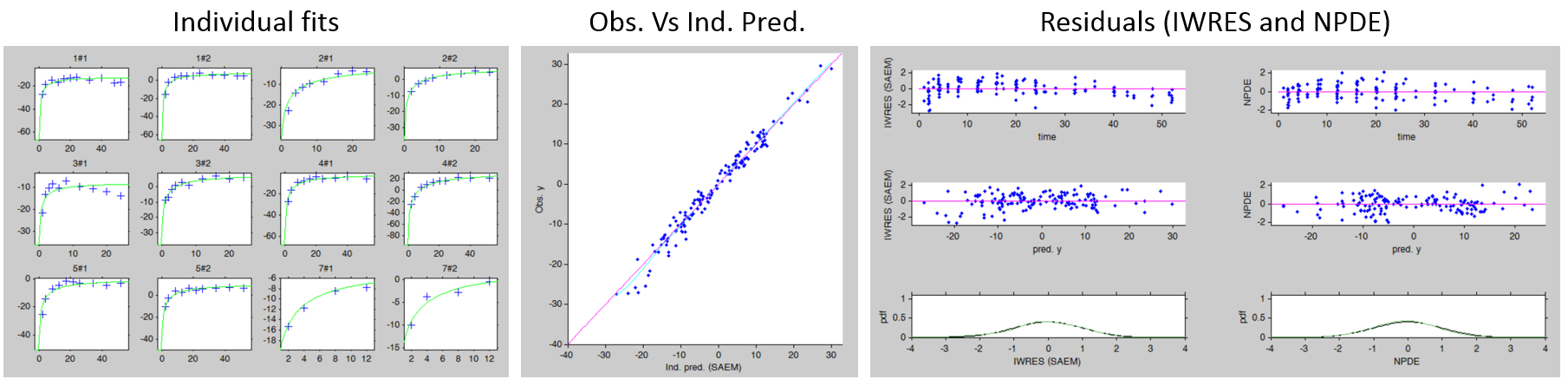
Note that all graphics use the transformed observations and transformed predictions.

Alternate models

One could try a more complex model including BSV and BTAV on T50 also. We leave this investigation as hands-on for the reader. The results are the following: the difference in AIC and BIC between the 2 models is small and some standard errors of the more complex model are unidentifiable. We thus decide to keep the simpler model.

Covariate search

The between study variability originates from the different inclusion criteria from study to study. To try to explain part of this variability, we can test adding the studied population characteristics as covariates. The available population characteristics are the mean number of swollen joints, the mean C-reactive protein level and the mean disease duration.
As these covariates differ between arms, they appear in the IOV window. We first transform the covariates using a reference value:

transformations

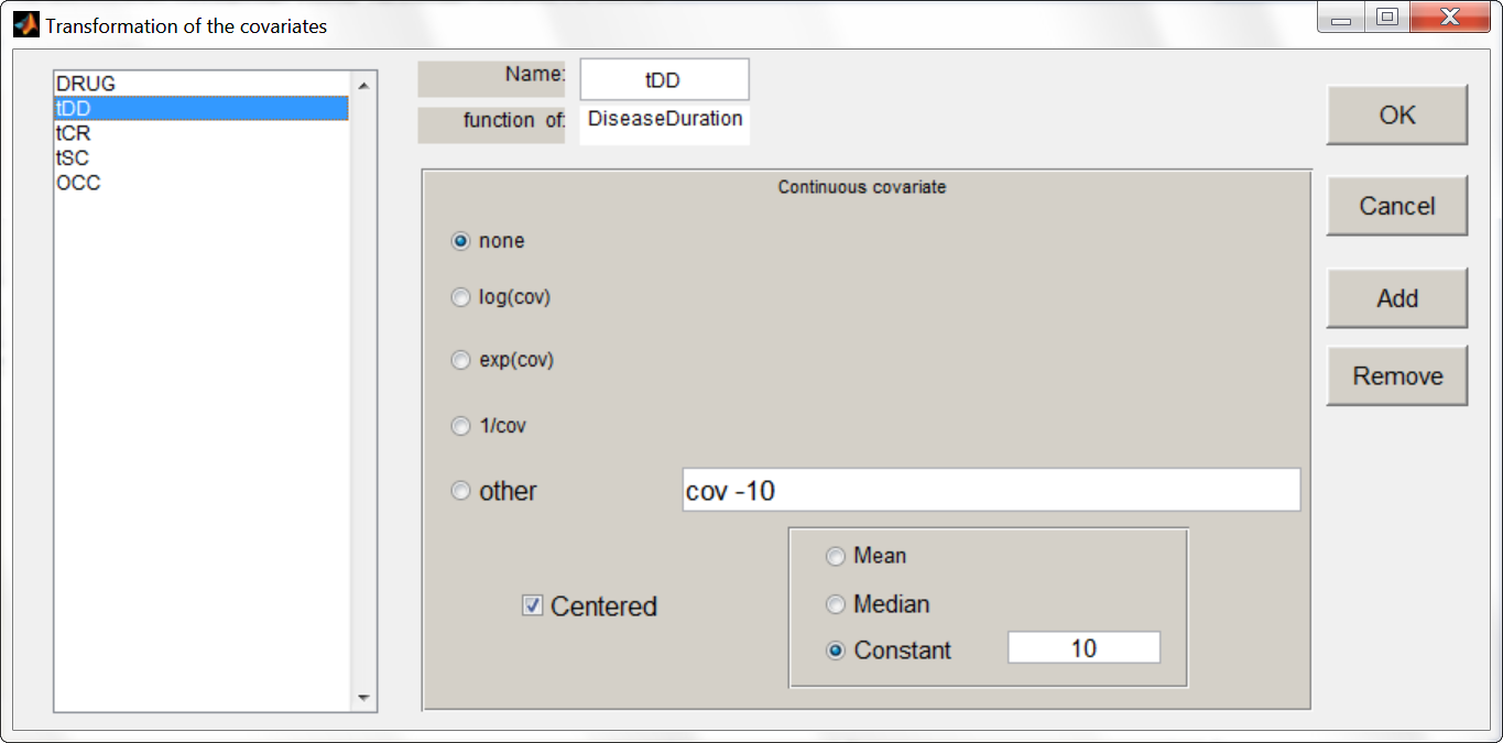
We then include them one by one in the model on the Emax parameter. We can either assess their significance using a Wald test (p-value in the result file, calculated with the Fisher Information Matrix Task), or a likelihood ratio. The advantage of the Wald test is that it requires only one model to be estimated (the one with the covariate) while the likelihood ratio requires both models (with and without covariate) to be estimated. The p-values of the Wald test testing if the beta’s are zero are:

Disease duration: p-value=0.76 (not significant)
C-reactive protein level: p-value=0.33 (not significant)
Swollen joint count: p-value=0.58 (not significant)

The likelihood ratio test also indicates that none of these covariates is significant. We thus do not include these covariates in the model.

Final model overview

The final model has an Emax structural model, with between study and between treatment arm variability on Emax, and no variability on T50. No covariates are included. One Emax and one T50 population parameter per type of treatment (placebo, abata, adali and canaki) is estimated (via the beta parameters).

Click here to download the Monolix projects.

Simulations for decision support

Comparison of canaki efficacy with drugs on the market

We now would like to use the developed model to compare the efficacy of Canaki with the efficacy of Abata and Adali. Has Canaki a chance to be more effective? To answer this question, we will perform simulations using simulx, the simulation function of the mlxR R package, which is based on the same calculation engine as Monolix.

To compare the true efficacy (over an infinitely large population) of Canaki with Abata and Adali, we could simply compare the Emax values. However the Emax estimates are marred with uncertainty, and this uncertainty should be taken into account. We will thus perform a large number of simulations for the 3 treatments, drawing the Emax population value from its uncertainty distribution. The BSV, BTAV and residual error are removed from the model because we now consider an infinitely large population, to focus on the “true efficacy”.

Before running a simulation, we need to define: the model, the population parameter values, the output (what we observe and at which time points), and the treatment type (Abata, Adali, Canaki or placebo).

Without the BSV and BTAV, the model is rewritten in the following way. It can either be provided as a separate file, or directly in the R script using the inlineModel function of the mlxR package:

ACR20model <-inlineModel("
[LONGITUDINAL]
input = {Emax, T50}

EQUATION:
ACR20 = Emax * (t / (T50 + t))
 
[COVARIATE]
input = {tDRUG}
tDRUG = {type=categorical, categories={abata, adali, canaki, placebo}}
 
[INDIVIDUAL]
input = {Emax_pop, beta_Emax_tDRUG_abata, beta_Emax_tDRUG_adali, beta_Emax_tDRUG_canaki, tDRUG, 
T50_pop, beta_T50_tDRUG_abata, beta_T50_tDRUG_adali, beta_T50_tDRUG_canaki}
tDRUG = {type=categorical, categories={abata, adali, canaki, placebo}}
 
DEFINITION:
Emax = {distribution=logitnormal, typical=Emax_pop, covariate=tDRUG, 
coefficient={beta_Emax_tDRUG_abata, beta_Emax_tDRUG_adali, beta_Emax_tDRUG_canaki, 0}, no-variability}
T50 = {distribution=lognormal, typical=T50_pop, covariate=tDRUG, 
coefficient={beta_T50_tDRUG_abata, beta_T50_tDRUG_adali, beta_T50_tDRUG_canaki, 0}, no-variability}
")

The estimated parameter values can either be directly written in a vector, or more conveniently read from the Monolix output file. A few additional lines are necessary to remove the supernumerary blanks in the parameter names and store the values in a named vector “param”:

populationParameter <- read.table('./project_03_mixed_withAnnea_1000iterFixed_/estimates.txt', 
header=TRUE, sep=';', col.names=c("name","value","sesa","relsesa","pval"))
name = as.character(populationParameter[[1]])
name = sub(" +", "", name)
name = sub(" +$", "", name)
param <- as.numeric(as.character(populationParameter[['value']]))
names(param) <- name

We next define the output. In Monolix we were working with the transformed prediction because of the constraints on the error model. As here we neglect the error model, we can directly output the (untransformed) ACR20, every week:

out <- list(name='ACR20',time=seq(0,52,by=1))

We then need to define the applied treatments, that appear in the model as a categorical covariate. As a first step, we simulate the ACR20 of each treatment using the estimated Emax and T50 values and neglecting the uncertainty. We thus define 4 individuals (i.e studies), one with each treatment:

covariates <- data.frame(id=1:4, tDRUG=c('abata','adali','canaki','placebo'))

All the information is then passed to the simulx function, for simulation. The results are stored in the R object “res”.

res <- simulx(model=myModel, parameter=list(covariates,param), output = out)

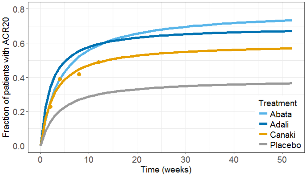
The results can then be plotted, together with the original Canaki data (dots), using usual R functions:

simulx1

We next would like to calculate a prediction interval for the true effect, taking into account the parameter uncertainty. Using the simpopmlx function of the mlxR package, we can easily draw population parameters from the correlation matrix:

# number of studies simulated for each of the three drugs, to take into account the uncertainty
NBstudy <- 1000

# we will use simpopmlx to draw population parameters, taking into account the correlations
paramWithUncertainty <- simpopmlx(n=4*NBstudy, project='./final_project.mlxtran')
colnames(paramWithUncertainty)[1] <- "id"

The output and covariate definition, as well as the simulation, is similar to the previous case:

 # define outputs
out <- list(name='ACR20',time=seq(0,52,by=1))
outc<- list(name='tDRUG')
# define covariates
covariates <- data.frame(id=1:(4*NBstudy), tDRUG=rep(c('abata','adali','canaki','placebo'),each=NBstudy))
#simulation
res2 <- simulx(model=myModel, parameter=list(covariates,paramWithUncertainty), output = list(out,outc))

After the simulation, the outputted data frames are slightly rearranged and plotted as 90% prediction interval using the prctilemlx function of the mlxR package:

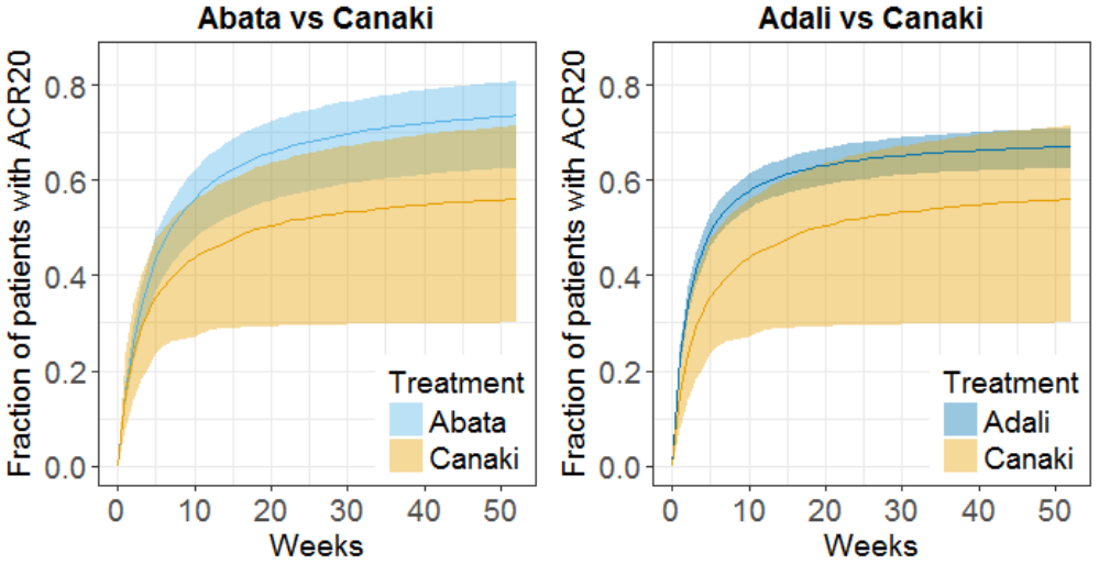
The prediction interval for Canaki is large, in accordance with its large uncertainty. Using the simulations, we calculate that:

at week 12, there are 8% chances that Canaki is better than Abata and 5% chances it is better than Adali
at week 52, there are 5.8% chances that Canaki is better than Abata and 15.6% chances it is better than Adali

We conclude that chances are low that the efficacy of Canaki is better than that of the drugs already on the market. In Demin et al., the authors conclude: “a decision was made not to pursue the RA indication. The integrated assessment of canakinumab data with the quantitative knowledge about current standard-of-care treatments supported this decision, given that the likelihood was low that canakinumab at current doses and regimen could provide incremental benefit to patients as compared with existing therapeutic options.“

For the purpose of this case study, we will continue with clinical trial simulations of a Canaki versus Placebo trial.

Simulations of a Canaki versus Placebo clinical trial

To simulate a clinical trial of Canaki versus Placebo, we this time need to take the BSV and BTAV into account, as well as the residual error, in addition to the uncertainty of the population parameters. The model code encompasses the structural model (section [LONGITUDINAL]) as in Monolix, but also the covariates (section [COVARIATE]) and the individual parameters distributions (section [INDIVIDUAL]), that in Monolix were defined via the GUI instead.
In addition, because simulx does not yet handle IOV, we define two etaBTAVEmax parameters in the [INDIVIDUAL] section, and use the first one for the first arm (occasion) and the second for the second arm (occasion). The arm index (0 for placebo and 1 for Canaki) is passed as regressor. The model is defined in the following:

Click here to see the Simulx model file

myModel <-inlineModel("
[LONGITUDINAL]
input = {Emax, T50, etaBSVEmax, etaBTAVEmax_OCCcanak,etaBTAVEmax_OCCplace, Narm, ARM, a}
Narm = {use=regressor}
ARM = {use=regressor}
EQUATION:
if ARM==0 ;ARM=0 corresponds to placebo
etaBTAVEmax = etaBTAVEmax_OCCplace
end
if ARM==1 ;ARM=1 corresponds to canaki
etaBTAVEmax = etaBTAVEmax_OCCcanak
end
; transform Emax to tEmax (normally distributed)
tEmax = logit(Emax)
; adding the random effects (RE) due to between-study variability and between arm variability,
; on the transformed parameters
tEmaxRE = tEmax + etaBSVEmax + etaBTAVEmax/sqrt(Narm)
; transforming back to have EmaxRE with logit distribution (values between 0 and 1)
EmaxRE = 1 / (1+ exp(-tEmaxRE) )
; defining the effect
ACR20 = EmaxRE * (t / (T50 + t))
; adding a saturation to avoid taking logit(0) (undefined) when t=0
ACR20sat = max(ACR20, 0.000001)
; transforming the effect ACR20 in the same way as the data
pred = logit(ACR20sat)*sqrt(Narm)

DEFINITION:
y= {distribution=normal, prediction=pred, sd=a}

[COVARIATE]
input = {tDRUG}
tDRUG = {type=categorical, categories={placebo, canaki}}

[INDIVIDUAL]
input = {Emax_pop, beta_Emax_tDRUG_canaki, tDRUG, T50_pop, beta_T50_tDRUG_canaki,
omega_etaBSVEmax, gamma_etaBTAVEmax}
tDRUG = {type=categorical, categories={placebo, canaki}}

DEFINITION:
Emax = {distribution=logitnormal, typical=Emax_pop, covariate=tDRUG,
coefficient={0, beta_Emax_tDRUG_canaki}, no-variability}
T50 = {distribution=lognormal, typical=T50_pop, covariate=tDRUG,
coefficient={0, beta_T50_tDRUG_canaki}, no-variability}
etaBSVEmax = {distribution=normal, typical=0, sd=omega_etaBSVEmax}
etaBTAVEmax_OCCcanak = {distribution=normal, typical=0, sd=gamma_etaBTAVEmax}
etaBTAVEmax_OCCplace = {distribution=normal, typical=0, sd=gamma_etaBTAVEmax}
")

All other simulx inputs are defined as before. After the simulation, we calculate the ACR20 back from the transformed prediction. We also calculate the standard deviation:

# transform the observation back to ACR20 observation
res3$y$ObsEffect <- 1/(1+exp(-1*res3$y$y/sqrt(Narm)))
# calculate the standard deviation 
res3$y$sd <- sqrt(1/Narm * res3$y$ObsEffect * (1-res3$y$ObsEffect))

The clinical trial simulation is plotted below:

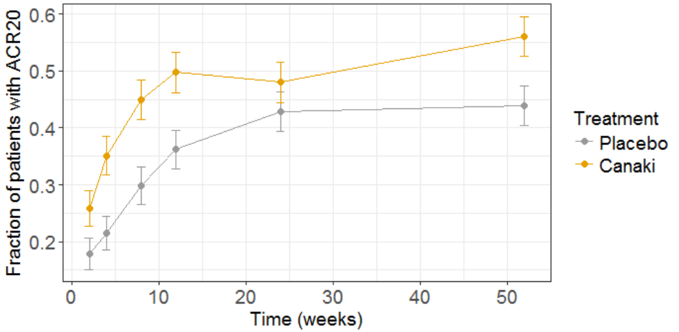
To test if Canaki is significantly more efficient than placebo, we can test if the proportion of patient at week 52 reaching ACR20 with Canaki is significantly higher than the fraction with placebo. For this, we perform a proportion test, using the R prop.test() function:

# test for proportion at week 52
NbPlacebo=w52$ObsEffect[1]*Narm
NbCanaki=w52$ObsEffect[2]*Narm
prop.test(x=c(NbPlacebo,NbCanaki),n=c(Narm,Narm),alternative="less")

The resulting p-value is 0.009, so we can consider that in this simulated clinical trial, Canaki turns out to be significantly more effective than placebo.

If we redo the simulation, sometimes the difference will not be significative. To know what our chances are to get a successful trial (i.e the power of the study), we can simulate a large number of trials and count in how many cases the trial would have been successful. Here we would like to know how the power of the study changes as we include more patients in the trial. To do so, we simulate 1000 studies with 4 different numbers of patients (50, 100, 200 or 400). We then calculate the power of the study in the following way:

nbSuccessFullTrials=0
for(k in 1:length(dfCanak$id)){
 tt <- prop.test(x=c(dfPlace$ObsEffect[k],dfCanak$ObsEffect[k])*Narm[i],n=rep(Narm[i],2), alternative="less")
 if(tt$p.value<0.05){
 nbSuccessFullTrials=nbSuccessFullTrials+1
 }
}
PowerStudy[i]=nbSuccessFullTrials/NBstudy

The results are the following:

Number of patients per arm	Power of the study
50	0.50
100	0.62
200	0.71
400	0.76

Thus, even if we recrute 400 patients per arm, the power of the study would only be around 75%.

All simulation scripts can be downloaded here.

Conclusion

Model-informed drug development

Model based meta-analysis supports critical decisions during the drug development process. In the present case, the model has shown that chances are low that Canaki performs better than two drugs already on the market. As a consequence the development of this drug has been stopped, thus saving the high costs of the phase III clinical trials. Clinical trial simulations based on a model can also be used to better design clinical trials. In the last section, we have for instance shown how to choose the number of patients per arm, in order to reach a predefined statistical power.

MBMA with Monolix and Simulx

This case study also aims at showing how Monolix and Simulx can be used to perform longitudinal model-based meta-analysis. Contrary to the usual parameter definition in Monolix, the weighting of the between treatment arm variability imposes to split the parameters into their fixed term and their BSV and BTAV terms, and reform the parameter in the model file. Once the logic of this model formulation is understood, the model set up becomes straightforward. The efficient SAEM algorithm for parameter estimation as well as the built in graphics then allow to efficiently analyze, diagnose and improve the model.
The inter-operability between Monolix and Simulx permits to carry the Monolix project over to Simulx to easily define and run clinical trial simulations. Several levels of variability/uncertainty (variability in covariates, variability in individual parameters, uncertainty in population parameters) can be included in an effortless way, either directly in the model file, or via auxiliary functions such as simpopmlx.

Natural extensions

In this case study, continuous data were used. Yet, the same procedure can be applied to other types of data such as count, categorical or time-to-event data.

Guidelines to implement your own MBMA model

Setting up your data set

Your data set should usually contain the following columns:

STUDY: index of the study/publication. It is equivalent to the ID column for individual-level data.
ARM: index of the arm (preferably continuous integers starting at 0). There can be an arbitrary number of arms (for instance several treated arms with different doses) and the order doesn’t matter. This column will be used as equivalent to the occasion OCC column.
TIME: time of the observations
Y: observations at the study level (percentage, mean response, etc)
transY: transformed observations, for which the residual error model is constant
Narm: number of individuals in the arm. Narm can vary over time
Covariates: continuous or categorical covariates that are characteristics of the study or of the arm. Covariates must be constant over arms (appear in IOV window) or over studies (appear in main window).

Frequent questions about the data set

Can dropouts (i.e. a time-varying number of individuals per arm) be taken into account? Yes. This can be accounted for without difficulty as the number of subjects per arm (Narm) is passed as a regressor to the model file, a type that allow by definition variations over time.
Can there be several treated (or placebo) arms per study? Yes. The different arms of a study are distinguished by a ARM index. For a given study, one can have observations for ARM=0, then observations for ARM=1, then observations for ARM=2. The index number has no special meaning (for instance ARM=0 can be the treated arm for study 1, and ARM=0 the placebo arm for study 2).
Why should I transform the observations? The observations must be transformed such that an error model from the list (constant, proportional, combined, exponential, etc) can be used. In the example above, we have done two transformations: first we have used a logit transformation, such that the prediction of the fraction of individuals reaching ACR20 will remain in the 0-1 interval, even if by chance a large residual error term is drawn. If we instead consider a mean concentration of glucose for instance, we could use a log-transformation to ensure positive values. Second, we need to multiply each value by the square root of the number of individuals per arm. With this transformation, the standard deviation of the error term is the same for all studies and arms, and does not depend on the number of individuals per arm anymore.

Setting up your model

The set up of your project can be done in four steps

Split the parameters in several terms
Make the appropriate transformation for the parameters
Set the parameter definition in the Monolix interface
Add the transformation of the prediction

Frequently asked questions on setting up the model

Why should I split a parameter in several terms? Because the standard deviation of the BTAV term must usually by weighted by the square root of the number of individuals per arm, this term must be handled as a separate parameter and added to the fixed effect within the model file. Moreover, the fixed effect and its BSV random effect might be split depending on the covariate definition.
How do I know in how many terms should I split my parameter?
- If all covariates of interest are constant over studies: 2. In this case, the parameters can be split into a (fixed effect + BSV) term and a (BTAV) term. The model file would for instance be (for a logit distributed parameter):
```
[LONGITUDINAL]
input = {paramFE_BSV, etaBTAVparam, Narm}
Narm = {use=regressor}
EQUATION:
tparam = logit(paramFE_BSV)
tparamRE = tparam + etaBTAVparam/sqrt(Narm)
paramRE = 1 / (1+ exp(-tparamRE))
```
  => Impact on the interface: In the GUI, paramFE_BSV would have both a fixed effect and a BSV random effect. Covariates can be added on this parameter in the main window. The etaBTAVparam fixed effect should be enforced to zero, the BSV disabled and the BTAV in the IOV window enabled.
- If one covariate of interest is not constant over studies: 3. This was the case for our case study (the DRUG covariates was constant over arms, not studies). Here, the parameters must be split into a fixed effect term, a BSV term and a BTAV term. The model file would for instance be (for a logit distributed parameter):
```
[LONGITUDINAL]
input = {paramFE, etaBSVparam, etaBTAVparam, Narm}
Narm = {use=regressor}
EQUATION:
tparam = logit(paramFE)
tparamRE = tparam + etaBSVparam + etaBTAVparam/sqrt(Narm)
paramRE = 1 / (1+ exp(-tparamRE))
```
  => Impact on the interface In the GUI, paramFE has only a fixed effect (BSV random effect must be disabled in the variance-covariance matrix). Covariates can be added on this parameter in the IOV window. The fixed effect value of etaBSVparam must be enforced to zero. The etaBTAVparam fixed effect should be enforced to zero too, the BSV disabled and the BTAV in the IOV window enabled.
Why shouldn’t I add covariates on the etaBTAVparam in the IOV window? Covariates can be added on etaBTAVparam in the IOV window. Yet, because the value of etaBTAVparam will be divided by the square root of the number of individuals in the model file, the covariate values in the data set must be transformed to counter-compensate. This may not always be feasible:
- If the covariate is categorical (as the DRUG on our example), it is not possible to compensate and thus the user should not add the covariate on the etaBTAVparam in the GUI. A splitting in 3 terms is needed.
- If the covariate is continuous (weight for example), it is possible to counter-compensate. Thus, if you add the covariates on the etaBTAVparam in the GUI, the covariate column in the data set must be multiplied by $\sqrt{N_{ik}}$ beforehand. This is a drawback, however this modeling has less parameters without variability and may thus converge more easily.

How should I transform the parameter depending on its distribution? Depending on the original parameter distribution, the parameter must first be transformed as in the following cases:

For a parameter with a normal distribution, called paramN for example, we would have done the following:

; no transformation on paramN as it is normally distributed
tparamN = paramN
; adding the random effects (RE) due to between-study and between arm variability, on the transformed parameter
tparamNRE = tparamN + etaBSVparamN + etaBTAVparamN/sqrt(Narm)
; no back transformation as tparamNRE already has a normal distribution
paramNRE = tparamNRE

Note that the two equalities are not necessary but there for clarity of the code.

For a parameter with a log-normal distribution, called paramLog for example (or T50 in the test case), we would have done the following:

; transformation from paramLog (log-normally distributed) to tparamLog (normally distributed)
tparamLog  = log(paramLog) 
; adding the random effects (RE) due to between-study and between arm variability, on the transformed parameter 
tparamLogRE = tparamLog  + etaBSVparamLog + etaBTAVparamLog/sqrt(Narm)
; transformation back to have paramLogRE with a log-normal distribution
paramLogRE = exp(tparamLogRE)

For a parameter with a logit-normal distribution, called paramLogit for example (or Emax in the test case), we would have done the following:

; transformation from paramLogit (logit-normally distributed) to tparamLogit (normally distributed)
tparamLogit  = logit(paramLogit) 
; adding the random effects (RE) due to between-study and between arm variability, on the transformed parameter 
tparamLogitRE = tparamLogit  + etaBSVparamLogit + etaBTAVparamLogit/sqrt(Narm)
; transformation back to have paramLogitRE with a logit-normal distribution
paramLogitRE = 1 / (1+ exp(-tparamLogitRE))

How do I set up the GUI? Depending which option has been chosen, the fixed effects and/or the BSV random effects and/or the BTAV random effects of the model parameters (representing one or several terms of the full parameter) must be enforced to 0. Random effects can be disabled to clicking on the diagonal terms of the variance-covariance matrix and fixed effects by choosing “fixed” after a right click.
Why and how do I transform the prediction? The model prediction must be transformed in the same way as the observations of the data set, using the column Narm passed as regressor.

Parameter estimation

The splitting of the parameters into several terms may introduce model parameters without variability. These parameters cannot be estimated using the main SAEM routine, but instead are optimized using alternative routines. Several of them are available in Monolix, under “Settings > Pop. parameters > Advanced > Zero-variability”. If the method by default leads to poor convergence, we recommend to test the other methods.

Model analysis

All graphics are displayed using the transformed observations and predictions. These are the right quantities to diagnose the model using the “Obs versus Pred” and “Residuals” graphics. For the individuals fits and VPC, it may also be interesting to look at the non-transformed observations and predictions. These graphics can be redone in R using the simulx function of the mlxR package. The other diagnostic plots (“Covariates”, “Parameters distribution”, “Random effects (boxplot)”, and “Random effects (joint)”) are not influenced by the transformation of the data.