- Model with continuous covariates
- Model with categorical covariates
- Transforming categorical covariates
Objectives: learn how to implement a model for continuous and/or categorical covariates.
Projects: warfarin_covariate1_project, warfarin_covariate2_project, warfarin_covariate3_project, phenobarbital_project
See also: Complex parameter-covariate relationships and time-dependent covariates
Model with continuous covariates
- warfarin_covariate1_project (data = ‘warfarin_data.txt’, model = ‘lib:oral1_1cpt_TlagkaVCl.txt’)
The warfarin data contains 2 individual covariates: weight which is a continuous covariate and sex which is a categorical covariate with 2 categories (1=Male, 0=Female). We can ignore these columns if are sure not to use them, or declare them using respectively the reserved keywords COV (for continuous covariate) and CAT (for categorical covariate):
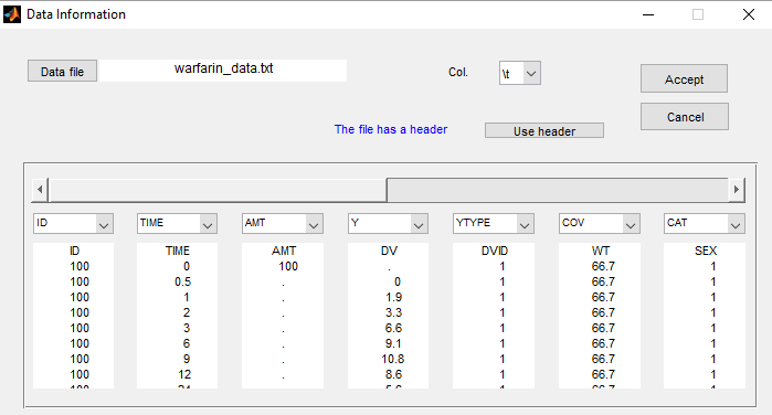
Even if these 2 covariates are now available, we can choose to define a model without any covariate:
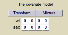
Here, a 0 on the first row (weight) and the third column (V), for instance, means that there is no relationship between weight and volume in the model. A diagnostic plot Covariates is generated which displays possible relationships between covariates and individual parameters (even if these covariates are not used in the model):
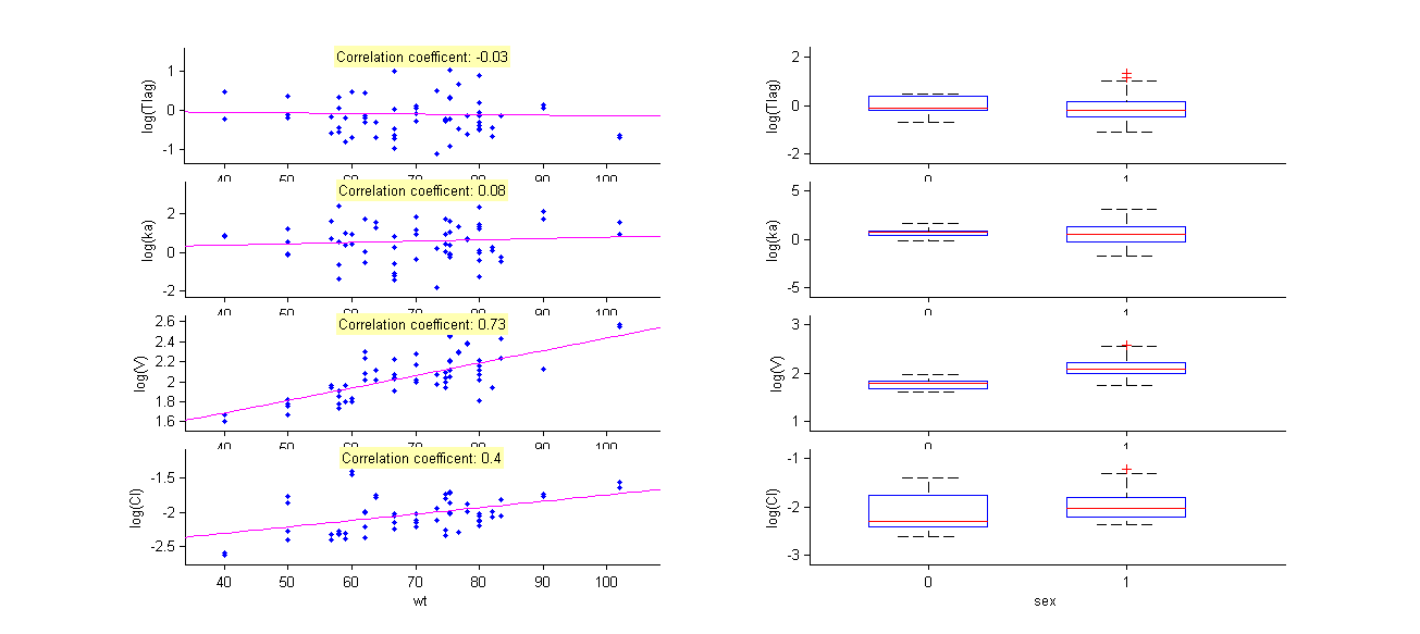
- warfarin_covariate2_project (data = ‘warfarin_data.txt’, model = ‘lib:oral1_1cpt_TlagkaVCl.txt’)
We decide to use the weight in this project in order to explain part of the variability of and
. We will implement the following model for these two parameters:
which means that population parameters of the PK parameters are defined for a typical individual of the population with weight=70kg.
More details about the model
The model for and
can be equivalently written as follows:
The individual predicted values for and
are therefore
and the statistical model describes how and
are distributed around these predicted values:
Here, and
are linear functions of
: we then need to transform first the original covariate
into
by clicking on the button
Transform of the main GUI. We can then transform and rename the original covariates of the dataset:
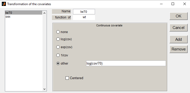
We then define a new covariate model, where and
are linear functions of the transformed weight
:
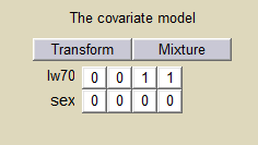
Coefficients and
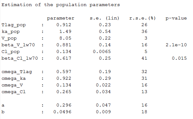
are now estimated with their s.e. and the p-values of the Wald tests are derived to test if these coefficients are different from 0:
Model with categorical covariates
- warfarin_covariate3_project (data = ‘warfarin_data.txt’, model = ‘lib:oral1_1cpt_TlagkaVCl.txt’)
We use sex instead of weight in this project, assuming different population values of volume and clearance for males and females.
More precisely, we consider the following model for and
:
where if individual
is a female and 0 otherwise. Then,
and
are the population volume and clearance for males while
and
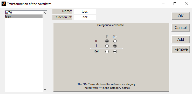
are the population volume and clearance for females. By clicking on the button
Transform, we can modify the name of the categories (click on the name of each category and enter a new name) and the reference category (Male is the reference category in this project):
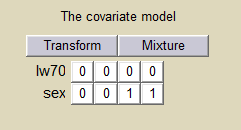
Define then the covariate model in the main GUI:
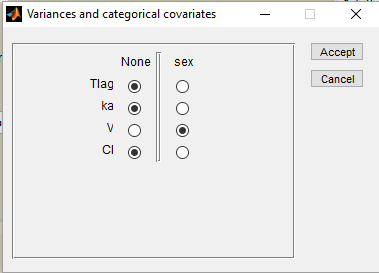
We can furthermore assume different variances of the random effects for males and females by clicking on the button
Cat. Var. and selecting which variances depend on the categorical covariate:
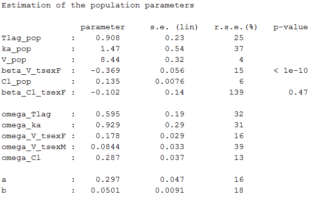
Estimated population parameters, including the coefficients and
and the 2 standard deviations
and
are displayed with the results:
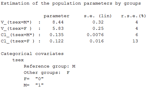
Estimated population parameters are also computed and displayed per category:
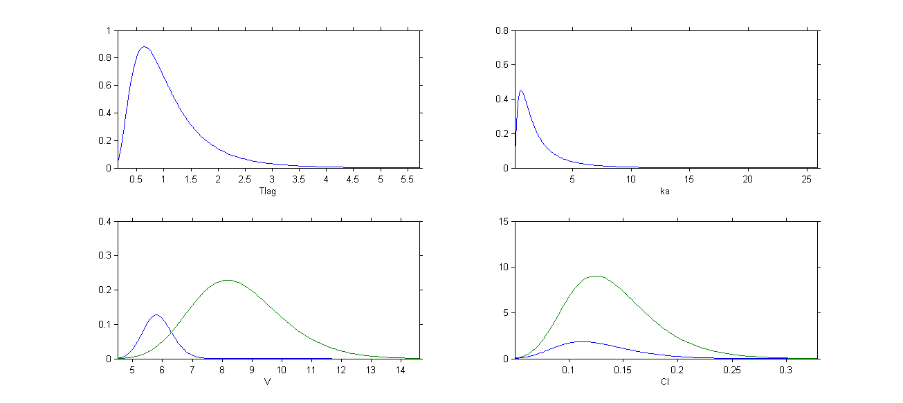
We can display the probability distribution functions of the 4 PK parameters:
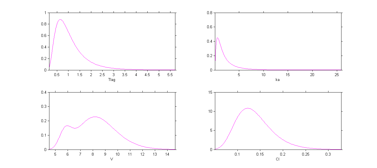
We can then distinguish the distributions for males and females by clicking on Settings and ticking the box By group:
Transforming categorical covariates
- phenobarbital_project (data = ‘phenobarbital_data.txt’, model = ‘lib:bolus_1cpt_Vk.txt’)
The phenobarbital data contains 2 covariates: the weight and the Apgar score which is considered as a categorical covariate:
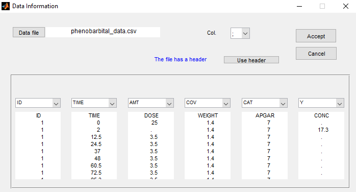
Instead of using the 10 original levels of the Apgar score, we will transform this categorical covariate and create 3 categories: Low = {1,2,3}, Medium = {4, 5, 6, 7} and High={8,9,10}.
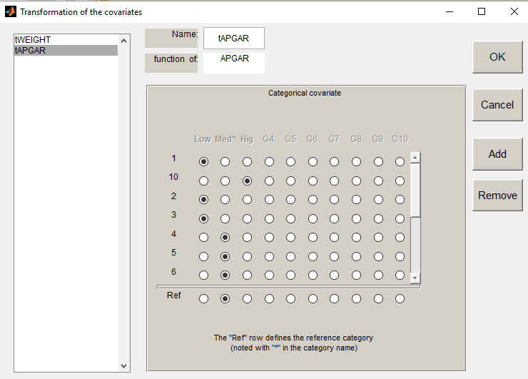
If we assume, for instance that the volume is related to the Apgar score, then and
are estimated (assuming that Medium is the reference level).