Objectives: learn how to implement a model for (repeated) time-to-event data with different censoring processes.
Projects: tte1_project, tte2_project, tte3_project, tte4_project, rtteWeibull_project, rtteWeibullCount_project
Introduction
Here, observations are the “times at which events occur”. An event may be one-off (e.g., death, hardware failure) or repeated (e.g., epileptic seizures, mechanical incidents, strikes). Several functions play key roles in time-to-event analysis: the survival, hazard and cumulative hazard functions. We are still working under a population approach here so these functions, detailed below, are thus individual functions, i.e., each subject has its own. As we are using parametric models, this means that these functions depend on individual parameters ")
- The survival function
gives the probability that the event happens to individual i after time
:
- The hazard function
is defined for individual i as the instantaneous rate of the event at time t, given that the event has not already occurred:
This is equivalent to
- Another useful quantity is the cumulative hazard function
, defined for individual i as
") gives the probability that the event happens to individual i after time
gives the probability that the event happens to individual i after time  :
:
 \ \ = \ \ \mathbb{P}(T_i>t;\psi_i) .")
 \ \ = \ \ \lim_{dt\to 0} \frac{S(t,\psi_i) - S(t + dt,\psi_i)}{ S(t,\psi_i) \, dt} .")
 \ \ = \ \ -\frac{d}{dt} \log{S(t,\psi_i)} .")
") , defined for individual i as
, defined for individual i as \ \ = \ \ \int_a^b h(t,\psi_i) \, dt .")
Note that  \ \ = \ \ e^{-H(t_{\text{start}},t;\psi_i)}")
")
")
Single event
To begin with, we will consider a one-off event. Depending on the application, the length of time to this event may be called the survival time (until death, for instance), failure time (until hardware fails), and so on. In general, we simply say “time-to-event”. The random variable representing the time-to-event for subject i is typically written Ti.
Single event exactly observed or right censored
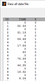
- tte1_project (data = tte1_data.txt , model=tte1_model.txt)
The event time may be exactly observed at time 


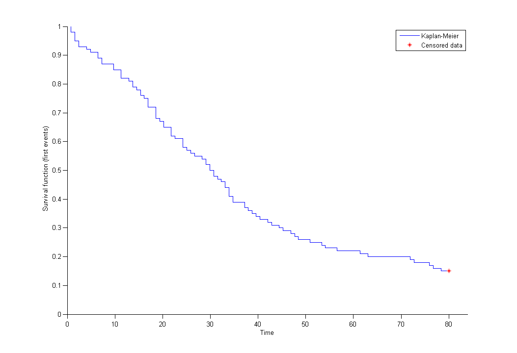
By clicking on the button plot the data, it is possible to display the Kaplan Meier plot (i.e. the empirical survival function) before fitting any model:
A very basic model with constant hazard is used for this data:
[LONGITUDINAL]
input = Te
DEFINITION:
Event = { type = event,  hazard = 1/Te,  maxEventNumber = 1 }
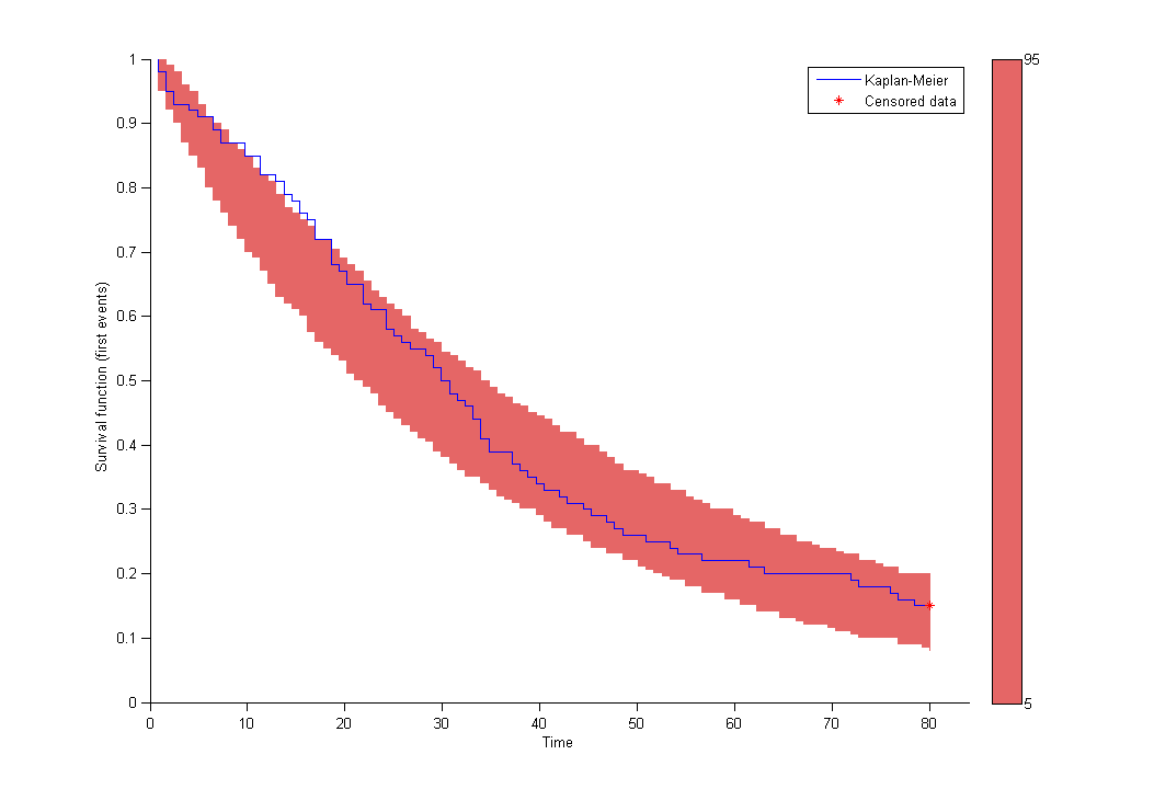
Here, Te is the expected time to event. Specification of the maximum number of events is required both for the estimation procedure and for the diagnostic plots based on simulation, such as the predicted interval for the Kaplan Meier plot which is obtained by Monte Carlo:
Single event interval censored or right censored
- tte2_project (data = tte2_data.txt , model=tte2_model.txt)
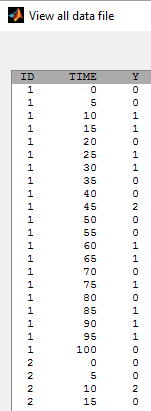
We may know the event has happened in an interval 
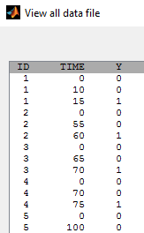
Event for individual 1 happened between t=10 and t=15. No event was observed until the end of the experiment (t=100) for individual 5. We use the same basic model, but we need now to specify that the events are interval censored:
[LONGITUDINAL]
input = Te
DEFINITION:
Event = {type=event,
         hazard=1/Te,
         eventType=intervalCensored,
         maxEventNumber=1,
         intervalLength=5,       ; used for the graphics (not mandatory)
         rightCensoringTime=200  ; used for the graphics (not mandatory)
}
Repeated events
Sometimes, an event can potentially happen again and again, e.g., epileptic seizures, heart attacks. For any given hazard function h, the survival function S for individual i now represents the survival since the previous event at 

 &=& \mathbb{P}(T_{i,j} > t_{i,j}\,|\,T_{i,j-1} = t_{i,j-1};\psi_i)\\&=&\exp(-H(t_{i,j-1},t_{i,j};\psi_i)) \\ &=&\exp(-\int_{t_{i,j-1}}^{t_{i,j}}h(t,\psi_i) dt) \end{array}")
Repeated events exactly observed or right censored
- tte3_project (data = tte3_data.txt , model=tte3_model.txt)
A sequence of 

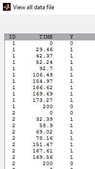
We can then display the Kaplan Meier plot for the first event and the mean number of events per individual:
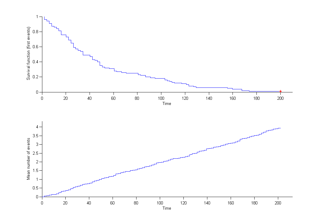
After fitting the model, prediction intervals for these two curves can also be displayed on the same graph.
Repeated events interval censored or right censored
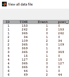
- tte4_project (data = tte4_data.txt , model=tte4_model.txt)
We do not know the exact event times, but the number of events that occurred for each individual in each interval of time:
User defined likelihood function for time-to-event data
- rtteWeibull_project (data = rtte_data.txt , model=rtteWeibull_model.txt)
A Weibull model is used in this example:
EQUATION:
h = (beta/lambda)*(t/lambda)^(beta-1)
DEFINITION:
Event = {type=event,  hazard=h}
- rtteWeibullCount_project (data = rtteCount_data.txt , model=rtteWeibullCount_model.txt)
Instead of defining the data as events, it is possible to consider the data as count data: indeed, we count the number of events per interval. An additional column with the start of the interval is added in the data file and defined as a regression variable:
We then use a model for count data (see rtteWeibullCount_model.txt).