Delayed differential equations

Ordinary differential equations based model
Don’t forget the initial conditions!
Delayed differential equations based model
Case studies

Objectives: learn how to implement a model with ordinary differential equations (ODE) and delayed differential equations (DDE).

Projects: tgi_project, seir_project, seir_noDelay_project

Ordinary differential equations based model

tgi_project (data = tgi_data.txt , model = tgi_model.txt)

We consider here the tumor growth inhibition (TGI) model proposed by Ribba *et al.* (Ribba, B., Kaloshi, G., Peyre, M., Ricard, D., Calvez, V., Tod, M., . & Ducray, F., *A tumor growth inhibition model for low-grade glioma treated with chemotherapy or radiotherapy*. Clinical Cancer Research, 18(18), 5071-5080, 2012.). This model is defined by a set of ordinary differential equations

$\begin{aligned}\frac{dC}{dt} &= - k_{de} C(t) \\\frac{dP_T}{dt} &= \lambda P_T(t)(1- P^{\star}(t)/K) + k_{QPP}Q_P(t) -k_{PQ} P_T(t) -\gamma \, k_{de} P_T(t)C(t) \\ \frac{dQ}{dt} &= k_{PK} P_T(t) -\gamma \, k_{de} Q(t)C(t) \\\frac{dQ_P}{dt} &= \gamma \, k_{de} Q(t)C(t) - k_{QPP} Q_P(t) -\delta_{QP} Q_P(t)\end{aligned}$

where $P^\star(t) = P_T(t) + Q(t) + Q_P(t)$ is the total tumor size. This set of ODEs is valid for $t>0$ , while

$\begin{aligned} C(t) &= 0 \\ P_T(t) &= P_{T0} \\ Q(t) &= Q_0 \\ Q_P(t) &= 0 \end{aligned}$

for $t \leq 0$ .This model (derivatives and initial conditions) can easily be implemented with Mlxtran:

[LONGITUDINAL]
input = {K, KDE, KPQ, KQPP, LAMBDAP, GAMMA, DELTAQP, PT0, Q0}
PK:
depot(target=C)
EQUATION:
t0=0
PT_0=PT0
Q_0 = Q0
PSTAR = PT+Q+QP
ddt_C = -KDE*C
ddt_PT = LAMBDAP*PT*(1-PSTAR/K) + KQPP*QP - KPQ*PT - GAMMA*KDE*PT*C
ddt_Q = KPQ*PT - GAMMA*KDE*Q*C
ddt_QP = GAMMA*KDE*Q*C - KQPP*QP - DELTAQP*QP

Remark: t0, PT_0 and Q_0 are reserved keywords that define the initial conditions.

Then, the graphic of individual fits clearly shows that the tumor size is constant until $t=0$ and starts changing according to the model at $t=0$ .

Don’t forget the initial conditions!

tgiNoT0_project (data = tgi_data.txt , model = tgi1NoT0_model.txt)

The initial time $t_0$ is not specified in this example

[LONGITUDINAL]
input = {K, KDE, KPQ, KQPP, LAMBDAP, GAMMA, DELTAQP, PT0, Q0}
PK:
depot(target=C)
EQUATION:
PT_0=PT0
Q_0 = Q0
PSTAR = PT+Q+QP
ddt_C = -KDE*C
ddt_PT = LAMBDAP*PT*(1-PSTAR/K) + KQPP*QP - KPQ*PT - GAMMA*KDE*PT*C
ddt_Q = KPQ*PT - GAMMA*KDE*Q*C
ddt_QP = GAMMA*KDE*Q*C - KQPP*QP - DELTAQP*QP

Since $t_0$ is missing, Monolix uses the first time value encountered for each individual. If, for instance, the tumor size is computed for $t\geq -5$ for the individual fits, then $t_0=-5$ will be used for defining the initial conditions, which introduces a shift in the plot:

Conclusion: don’t forget to specify properly the initial conditions of a system of ODEs!

Delayed differential equations based model

A system of delay differential equations (DDEs) can be implemented in a block EQUATION of the section [LONGITUDINAL] of a script Mlxtran. Mlxtran provides the command delay(x,T) where x is a one-dimensional component and T is the explicit delay. Therefore, DDEs with a nonconstant past of the form

$\begin{array}{ccl} \frac{dx}{dt} &=& f(x(t),x(t-T_1), x(t-T_2), ...), ~~\text{for}~~t \geq 0\\ x(t) &=& x_0(t) ~~~~\text{for}~~\text{min}(T_k) \leq t \leq 0 \end{array}$

can be solved.

seir_project (data = seir_data.txt , model = seir_model.txt)

The model is a system of 4 DDEs:

[LONGITUDINAL]
input = {A, lambda, gamma, epsilon, d, tau, omega}
EQUATION:
t0 = 0
S_0 = 15
E_0 = 0
I_0 = 2
R_0 = 3
N = S + E + I + R
ddt_S = A - d*S - lambda*S*I/N + gamma*delay(I,tau)*exp(-d*tau)
ddt_E = lambda*S*I/N - d*E - lambda*delay(S,omega)*delay(I,omega)*exp(-d*omega)/(delay(I,omega) + delay(S,omega) + delay(E,omega) + delay(R,omega))
ddt_I = -(gamma+epsilon+d)*I + lambda*delay(S,omega)*delay(I,omega)*exp(-d*omega)/(delay(I,omega) + delay(S,omega) + delay(E,omega) + delay(R,omega))
ddt_R = gamma*I - d*R - gamma*delay(I,tau)*exp(-d*tau)

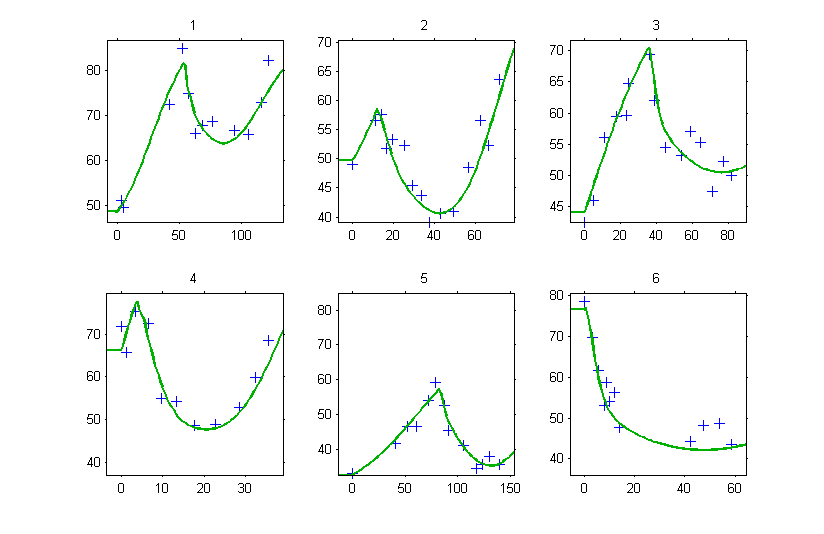
Introducing these delays allows to obtain nice fits for the 4 outcomes, including $(R_{ij})$ :

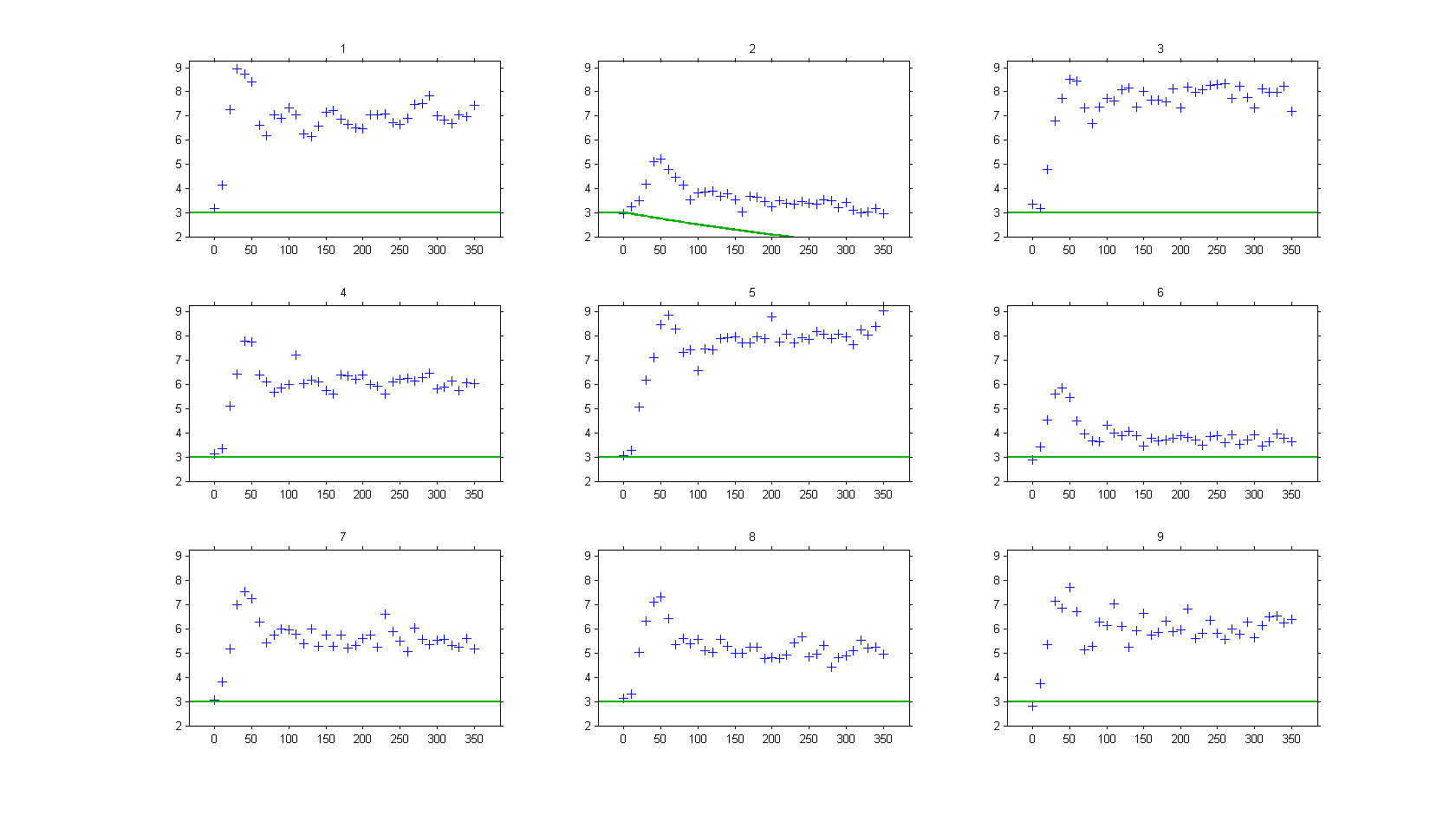
seir_noDelay_project (data = seir_data.txt , model = seir_model.txt)

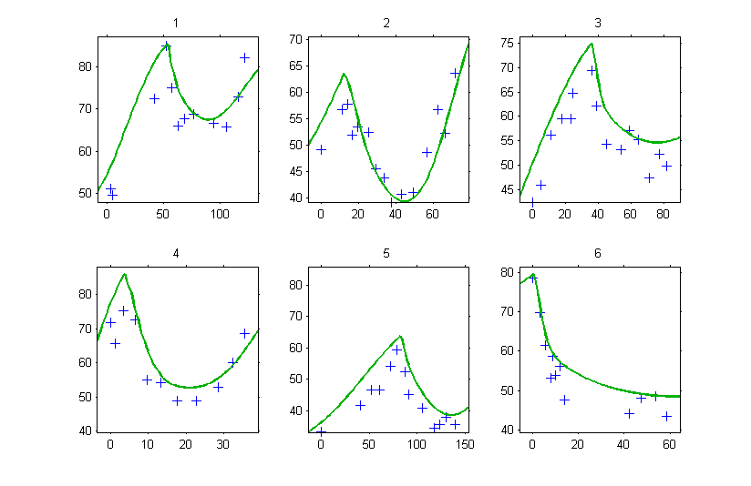
On the other hand, if ODEs are used, i.e. without any delay,

then, the model is not able anymore to fit correctly the observed data, such as $(R_{ij})$ :

Case studies

8.case_studies/arthritis_project