Count data model

Introduction
Count data with constant distribution over time
Count data with time varying distribution
Hidden Markov model for count data

Objectives: learn how to implement a model for count data.

Projects: count1a_project, count1a_project, count1a_project, count2_project, hmm0_project, hmm1_project

Introduction

Longitudinal count data is a special type of longitudinal data that can take only nonnegative integer values {0, 1, 2, …} that come from counting something, e.g., the number of seizures, hemorrhages or lesions in each given time period . In this context, data from individual j is the sequence $y_i=(y_{ij},1\leq j \leq n_i)$ where $y_{ij}$ is the number of events observed in the jth time interval $I_{ij}$ .
Count data models can also be used for modeling other types of data such as the number of trials required for completing a given task or the number of successes (or failures) during some exercise. Here, $y_{ij}$ is either the number of trials or successes (or failures) for subject i at time $t_{ij}$ . For any of these data types we will then model $y_i=(y_{ij},1\leq j \leq n_i)$ as a sequence of random variables that take their values in {0, 1, 2, …}. If we assume that they are independent, then the model is completely defined by the probability mass functions $\mathbb{P}(y_{ij}=k)$ for $k \geq 0$ and $1 \leq j \leq n_i$ . Here, we will consider only parametric distributions for count data.

Count data with constant distribution over time

count1a_project (data = ‘count1_data.txt’, model = ‘count_library/poisson_mlxt.txt’)

A Poisson model is used for fitting the data:

[LONGITUDINAL]
input = lambda
DEFINITION:
Y = { type = count,  log(P(Y=k)) = -lambda + k*log(lambda) - factln(k) }

Residuals for noncontinuous data reduce to NPDE’s. We can compare the empirical distribution of the NPDE’s with the distribution of a standardized normal distribution:

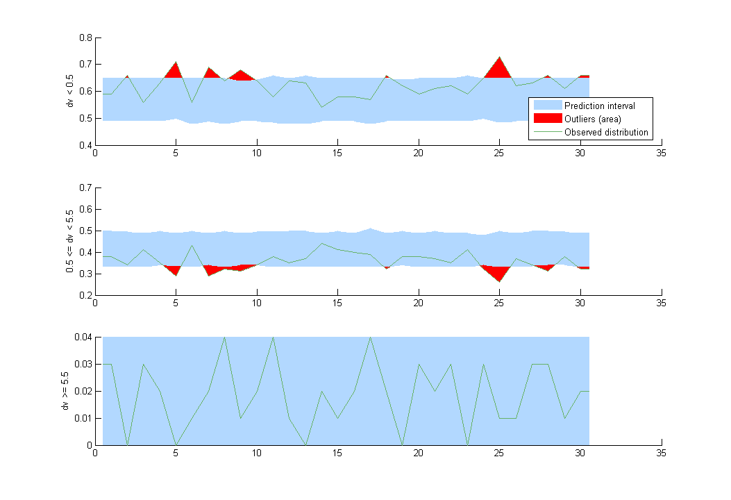
VPC’s for count data compare the observed and predicted frequencies of the categorized data over time:

count1b_project (data = ‘count1_data.txt’, model = ‘count_library/poissonMixture_mlxt.txt’)

A mixture of 2 Poisson distributions is used to fit the same data.

Count data with time varying distribution

count2_project (data = ‘count2_data.txt’, model = ‘count_library/poissonTimeVarying_mlxt.txt’)

The distribution of the data changes with time in this example:

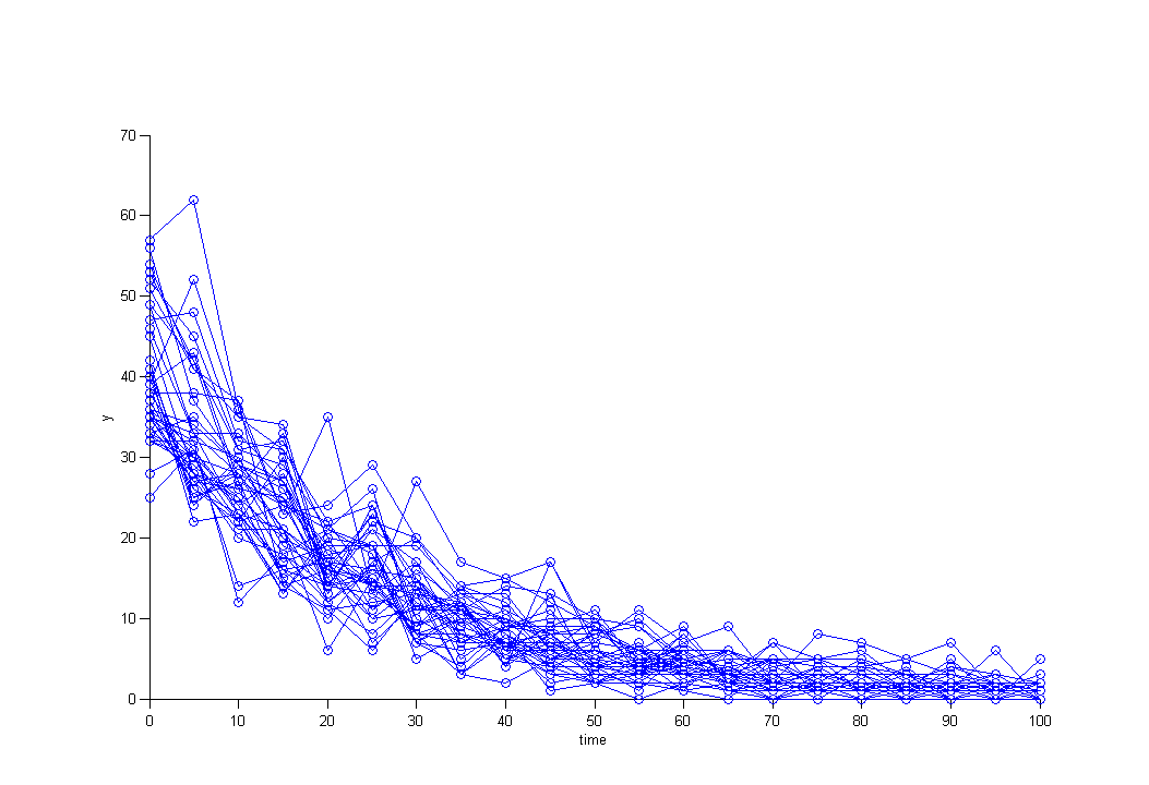
We then use a Poisson distribution with a time varying intensity:

[LONGITUDINAL]
input =  {a,b}
                           
EQUATION:
lambda= a*exp(-b*t)
                           
DEFINITION:
y = {type=count, P(y=k)=exp(-lambda)*(lambda^k)/factorial(k)}

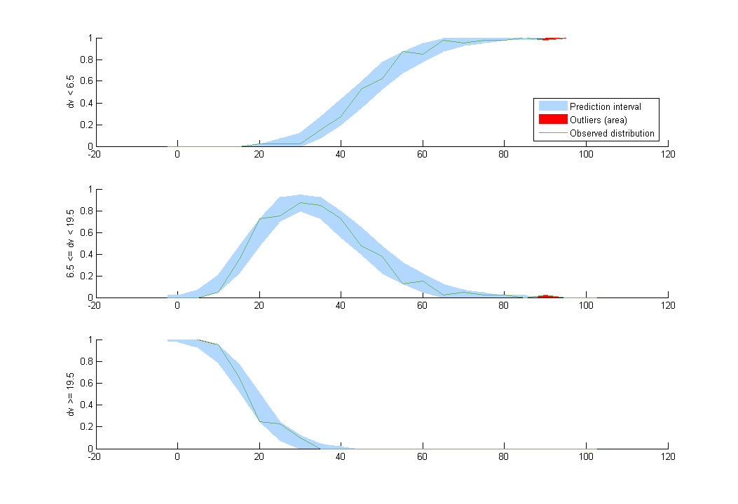
This model seems to fit the data very well:

Hidden Markov model for count data

Markov chains are a useful tool for analyzing categorical longitudinal data. However, sometimes the Markov process cannot be directly observed and only some output, dependent on the (hidden) state, is seen. More precisely, we assume that the distribution of this observable output depends on the underlying hidden state. Such models are called hidden Markov models. An HMM is thus defined for individual $i$ as a pair of processes $(z_{ij},y_{ij},\, j=1,2,\ldots)$ , where the latent sequence $(z_{ij})$ is a Markov chain and the distribution of observation $y_{ij}$ at time $t_{ij}$ depends on state $z_{ij}$ .
In the following example, the latent sequence $(z_{ij})$ take its values in $\{1, 2\}$ . When $z_{ij}=1$ (resp. $z_{ij}=2$ ), $y_{ij}$ is a Poisson random variable with parameter $\lambda_1$ (resp. $\lambda_2$ ).
Remark: Models in the 2 following examples are implemented in Matlab (implementation with Mlxtran is not possible with the current version of Monolix). These models can be used with both the StandAlone and Matlab versions of Monolix, but they can only be modified with the Matlab version.

hmm0_project (data = ‘hmm_data.txt’, model = ‘count_library/hmm0_mlx.m’)

The latent sequence $(z_{ij})$ is a sequence of independent and identically distributed random variables.

hmm1_project (data = ‘hmm_data.txt’, model = ‘count_library/hmm1_mlx.m’)

The latent sequence $(z_{ij})$ is a (hidden) Markov chain.