- Introduction
- Theory
- PK data below a lower limit of quantification
- PK data below a lower limit of quantification or below a limit of detection
- PK data below a lower limit of quantification and PD data above an upper limit of quantification
- Combination of interval censored PK and PD data
- Case studies
Objectives: learn how to handle easily and properly censored data, i.e. data below (resp. above) a lower (resp.upper) limit of quantification (LOQ) or below a limit of detection (LOD).
Projects: censored1log_project, censored1_project, censored2_project, censored3_project, censored4_project
Introduction
Censoring occurs when the value of a measurement or observation is only partially known. For continuous data measurements in the longitudinal context, censoring refers to the values of the measurements, not the times at which they were taken. For example, the lower limit of detection (LLOD) is the lowest quantity of a substance that can be distinguished from its absence. Therefore, any time the quantity is below the LLOD, the “observation” is not a measurement but the information that the measured quantity is less than the LLOD. Similarly, in longitudinal studies of viral kinetics, measurements of the viral load below a certain limit, referred to as the lower limit of quantification (LLOQ), are so low that their reliability is considered suspect. A measuring device can also have an upper limit of quantification (ULOQ) such that any value above this limit cannot be measured and reported.
As hinted above, censored values are not typically reported as a number, but their existence is known, as well as the type of censoring. Thus, the observation }_{ij}")

We usually distinguish between three types of censoring: left, right and interval. In each case, the SAEM algorithm implemented in Monolix properly computes the maximum likelihood estimate of the population parameters, combining all the infomation provided by censored and non censored data.
Theory
In the presence of censored data, the conditional density function needs to be computed carefully. To cover all three types of censoring (left, right, interval), let 

}|\psi)=\prod_{i=1}^{N}\prod_{j=1}^{n_i}p(y_{ij}|\psi_i)^{1_{y_{ij}\notin I_{ij}}}\mathbb{P}(y_{ij}\in I_{ij}|\psi_i)^{1_{y_{ij}\in I_{ij}}}")
where
=\int_{I_{ij}} p_{y_{ij}|\psi_i} (u|\psi_i)du")
We see that if 
")
")
For the calculation of the likelihood, this is equivalent to the M3 method in NONMEM when only the CENS column is given, and to the M4 method when both a CENS column and a LIMIT column are given.
PK data below a lower limit of quantification
Left censored data
- censored1log_project (data = ‘censored1log_data.txt’, model = ‘pklog_model.txt’)
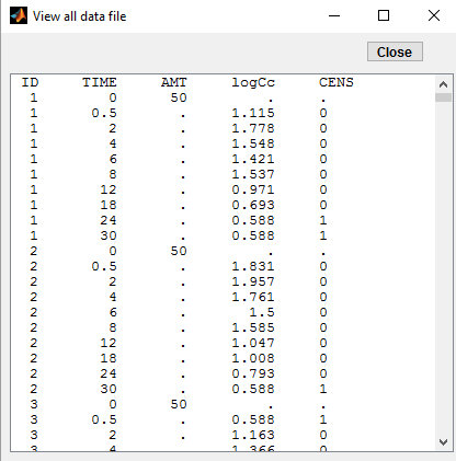
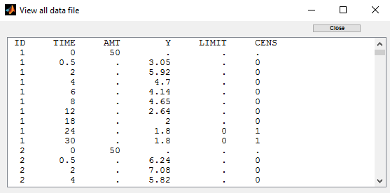
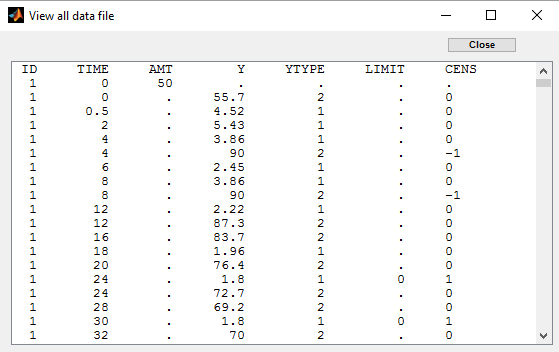
PK data are log-concentration in this example. The limit of quantification of 1.8 mg/l for concentrations becomes log(1.8)=0.588 for log-concentrations. Column of observations (Y) contains either the LLOQ for data below the limit of quantification (BLQ data) or the measured log-concentrations for non BLQ data. Furthermore, Monolix uses an additional column CENS to indicate if an observation is left censored (CENS=1) or not (CENS=0). In this example, subject 1 has two BLQ data at time 24h and 30h (the measured log-concentrations were below 0.588 at these times):
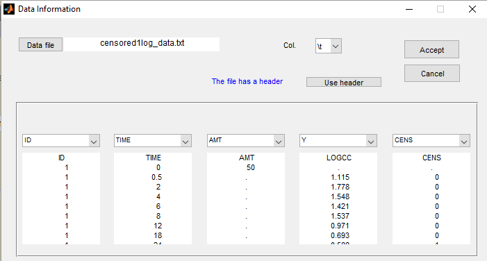
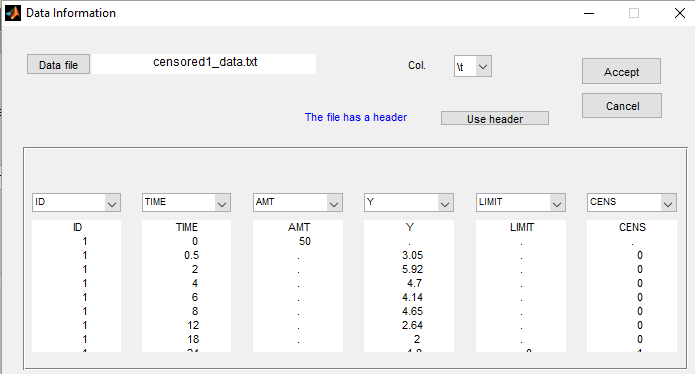
Monolix then recognized this keyword CENS:
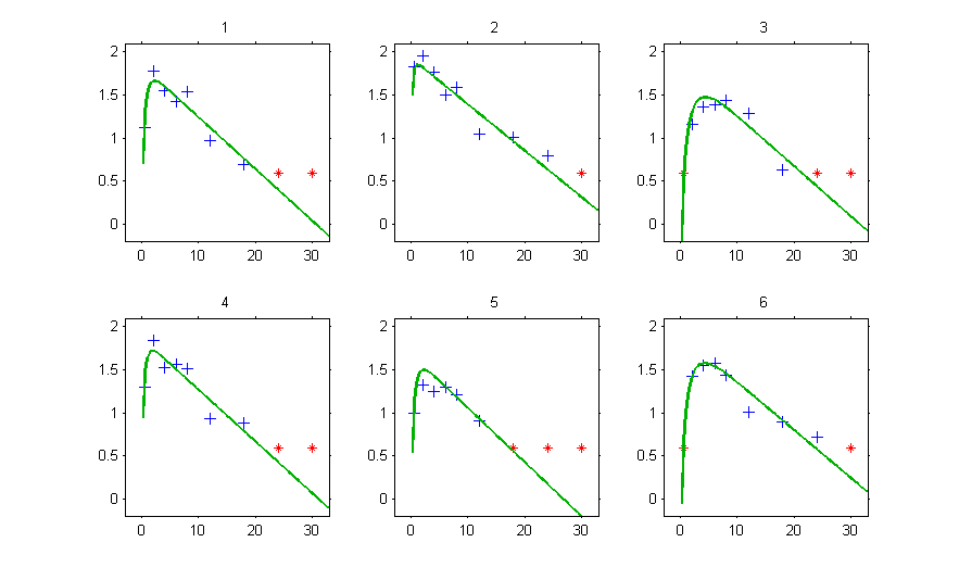
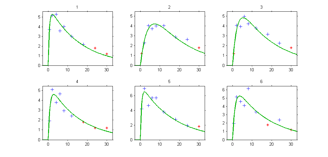
The plot of individual fits displays BLQ and non BLQ data together with the predicted log-concentrations on the whole time interval:
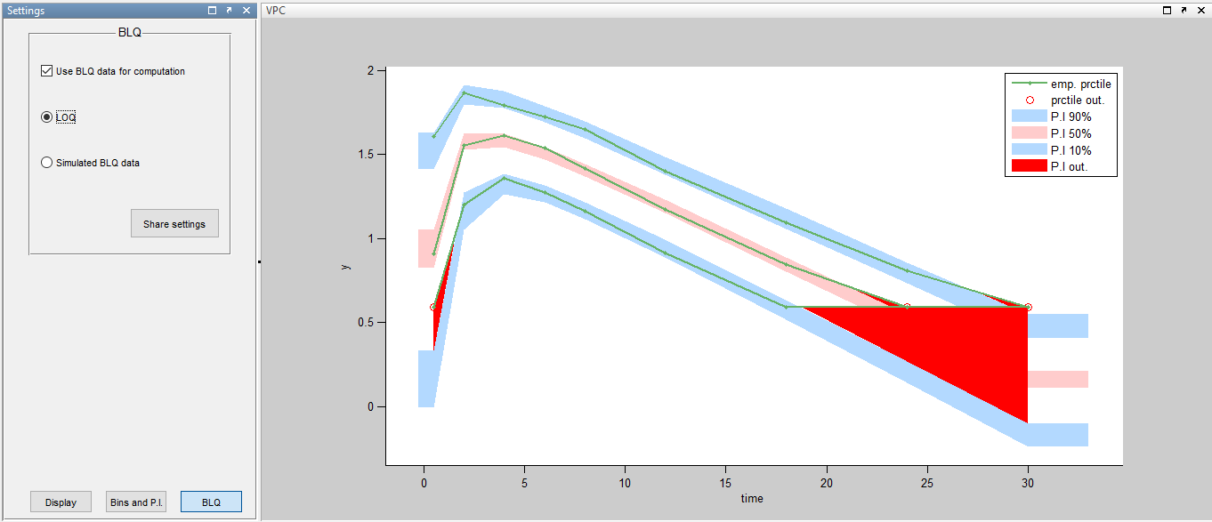
For diagnostic plots such as VPC, residuals of observations versus predictions, Monolix proposes to sample the BLQ data from the conditional distribution
")
where 

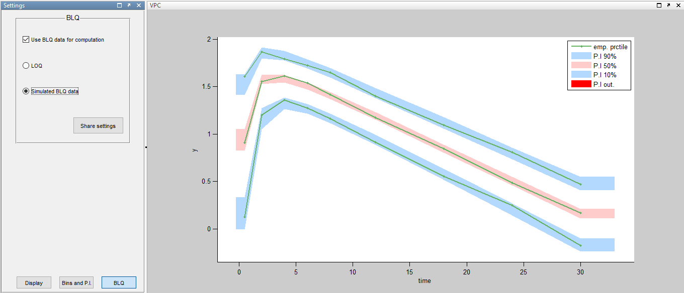
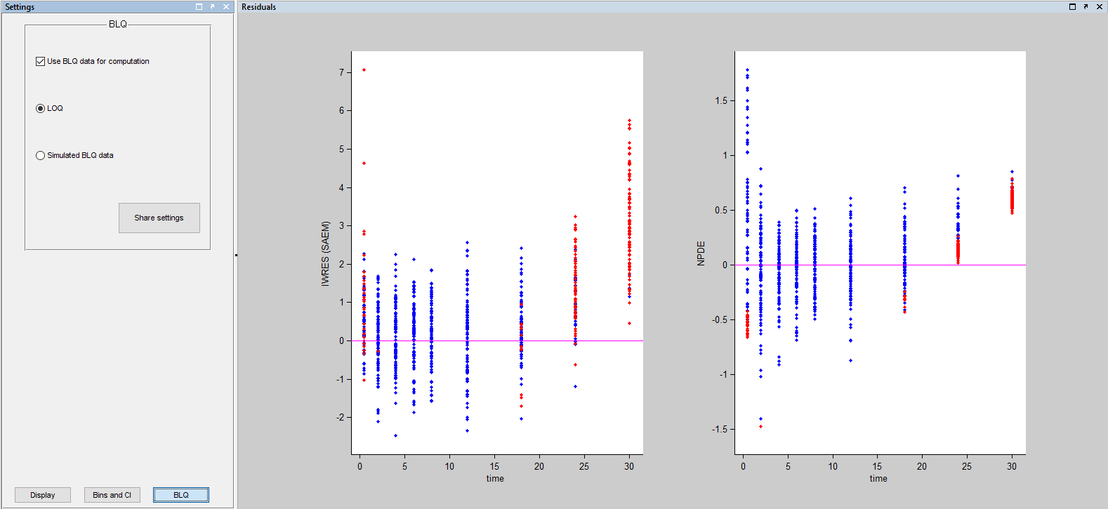
A strong bias appears if LLOQ is used instead for the BLQ data:
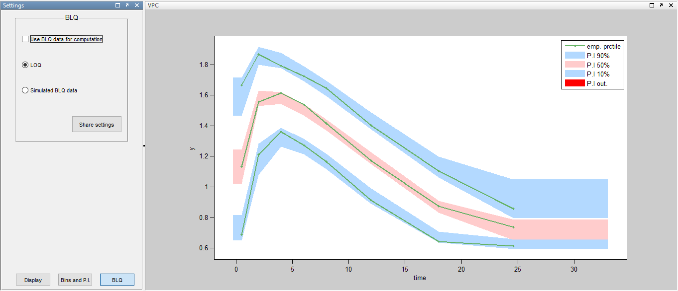
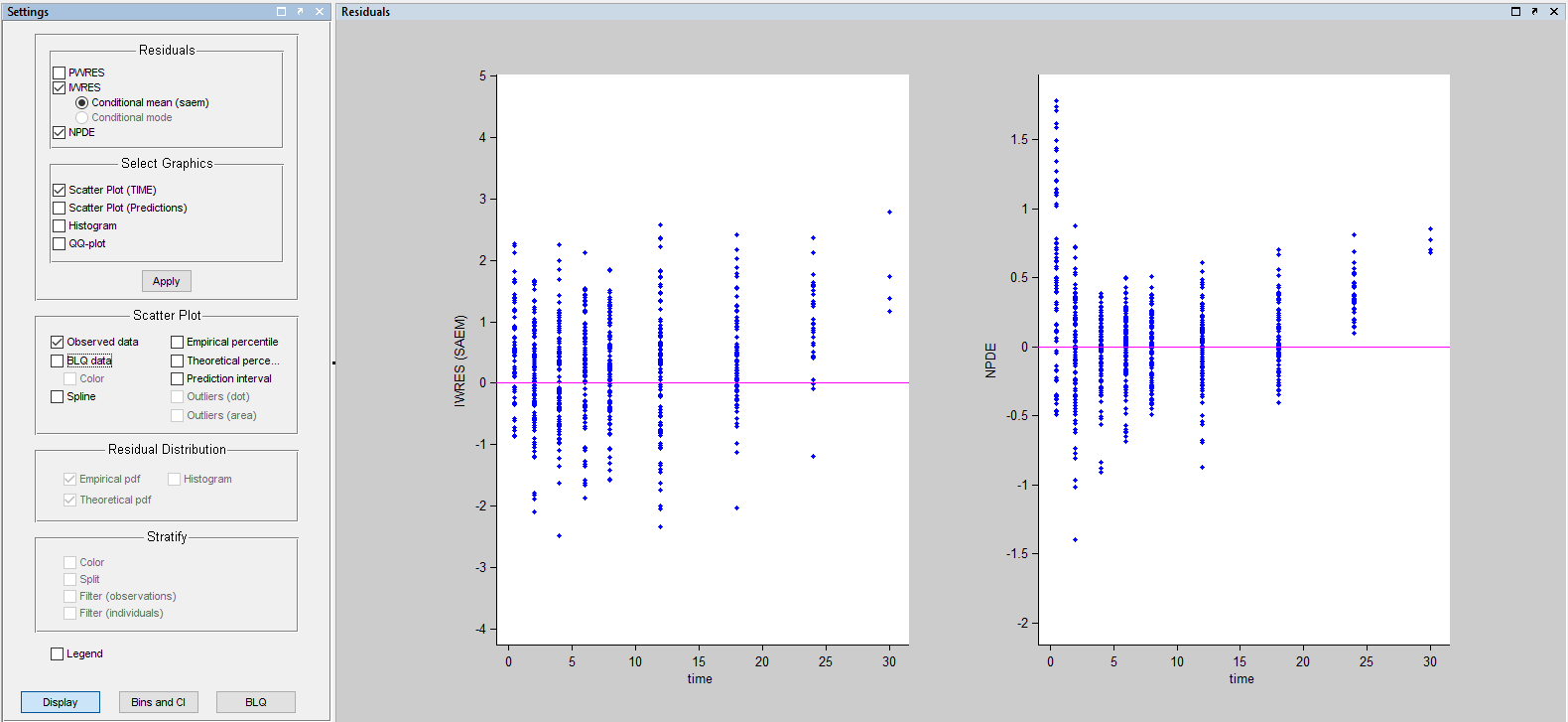
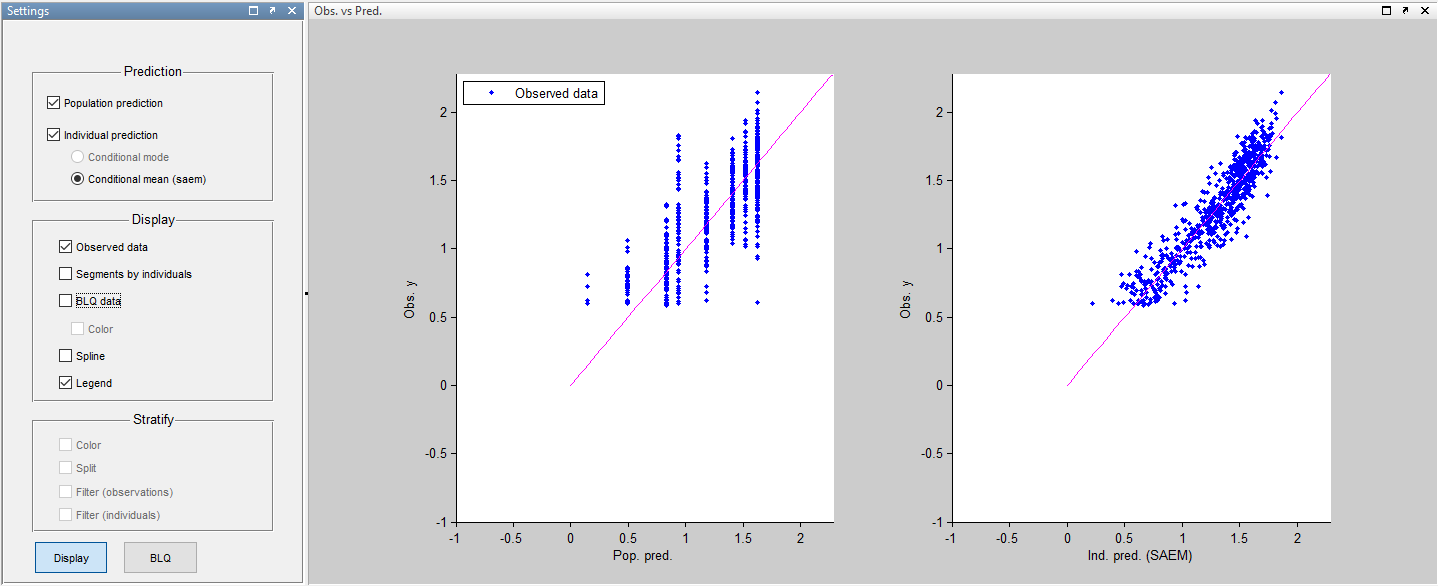
Ignoring the BLQ data entails a loss of information:
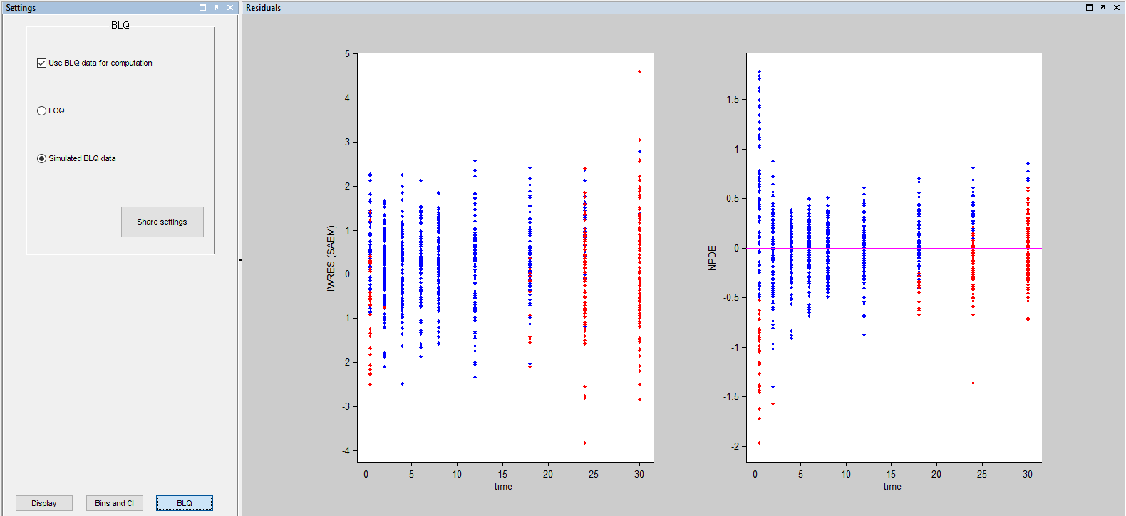
Imputed BLQ data is also used for residuals:
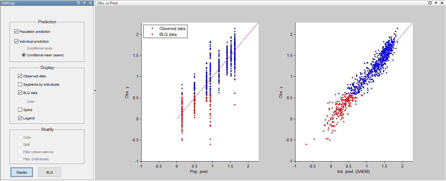
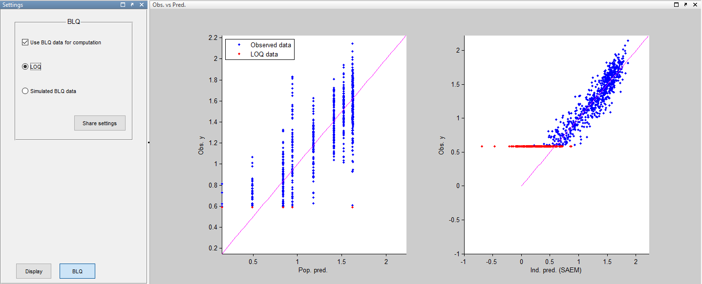
and for observations versus predictions:
More about these diagnostic plots
A strong bias appears if LLOQ is used instead for the BLQ data for these two diagnostic plots:
while ignoring the BLQ data entails a loss of information:
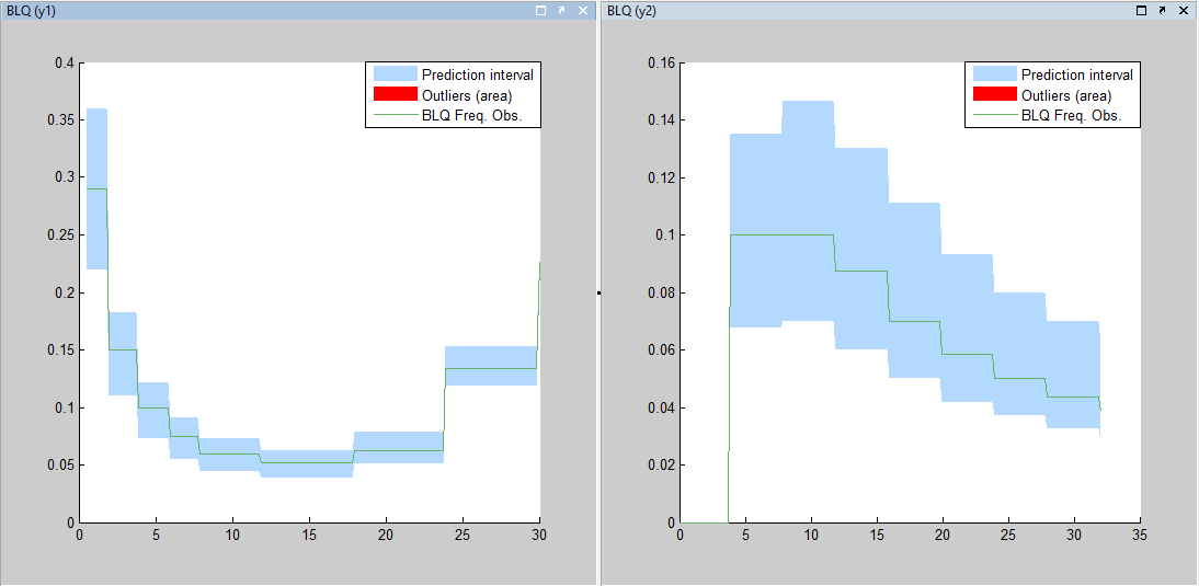
Diagnostic plot BLQ plots the cumulative fraction of BLQ data (green line) with a 90 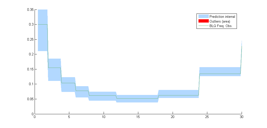
Interval censored data
- censored1_project (data = ‘censored1_data.txt’, model = ‘lib:oral1_1cpt_kaVk.txt’)
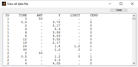
We use the original concentrations in this project. Then, BLQ data should be treated as interval censored data since a concentration is know to be positive. In other word, a data reported as BLQ data means that the (non reported) measured concentration is between 0 and 1.8mg/l. An additional column LIMIT reports the lower limit of the censored interval (0 in this example):
Remark: if this column is missing, then BLQ data is assumed to be left-censored data that can take any positive and negative value below LLOQ.
Monolix recognized this keyword LIMIT:
Monolix will use this additional information for properly estimating the parameters of the model and imputing the BLQ data for the diagnostic plots.
PK data below a lower limit of quantification or below a limit of detection
- censored2_project (data = ‘censored2_data.txt’, model = ‘lib:oral1_1cpt_kaVk.txt’)
Several censoring processes can be combined in the same data set, assuming different limits. We may know, for instance that a PK data is either below a limit of detection (
Plot of individual fits now displays LLOQ or LLOD with a red star when a PK data is censored:
PK data below a lower limit of quantification and PD data above an upper limit of quantification
- censored3_project (data = ‘censored3_data.txt’, model = ‘pkpd_model.txt’)
We work with PK and PD data in this project. We assume that the PD data may be right censored and that the upper limit of quantification is ULOQ=90. We use CENS=-1 to indicate that an observation is right censored. In such case, the PD data can take any value above the upper limit reported in column Y (here YTYPE=1 and YTYPE=2 are used respectively for PK and PD data):
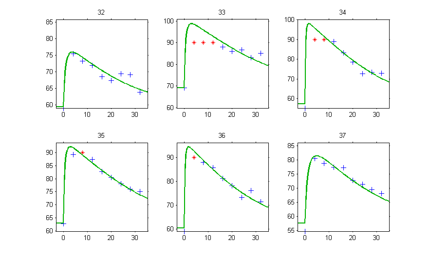
Plot of individual fits for the PD data now displays ULOQ and the predicted PD profile:
We can display the cumulated fraction of censored data both for the PK and the PD data:
Combination of interval censored PK and PD data
- censored4_project (data = ‘censored4_data.txt’, model = ‘pkpd_model.txt’)
We assume in this example
- 2 different censoring intervals(0,1) and (1.2, 1.8) for the PK,
- a censoring interval (80,90) and right censoring (>90) for the PD.
Combining columns CENS, LIMIT and Y allow to combine efficiently these different censoring processes:
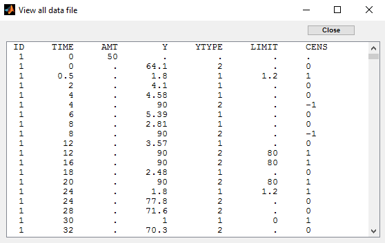
This coding of the data means that, for subject 1,
- PK data is between 0 and 1 at time 30h,
- PK data is between 1.2 and 1.8 at times 0.5h and 24h,
- PD data is between 80 and 90 at times 12 and 16,
- PD data is above 90 at times 4 and 8.
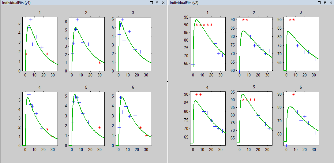
Plot of individual fits for the PK and the PD data displays the different limits of these censoring intervals:
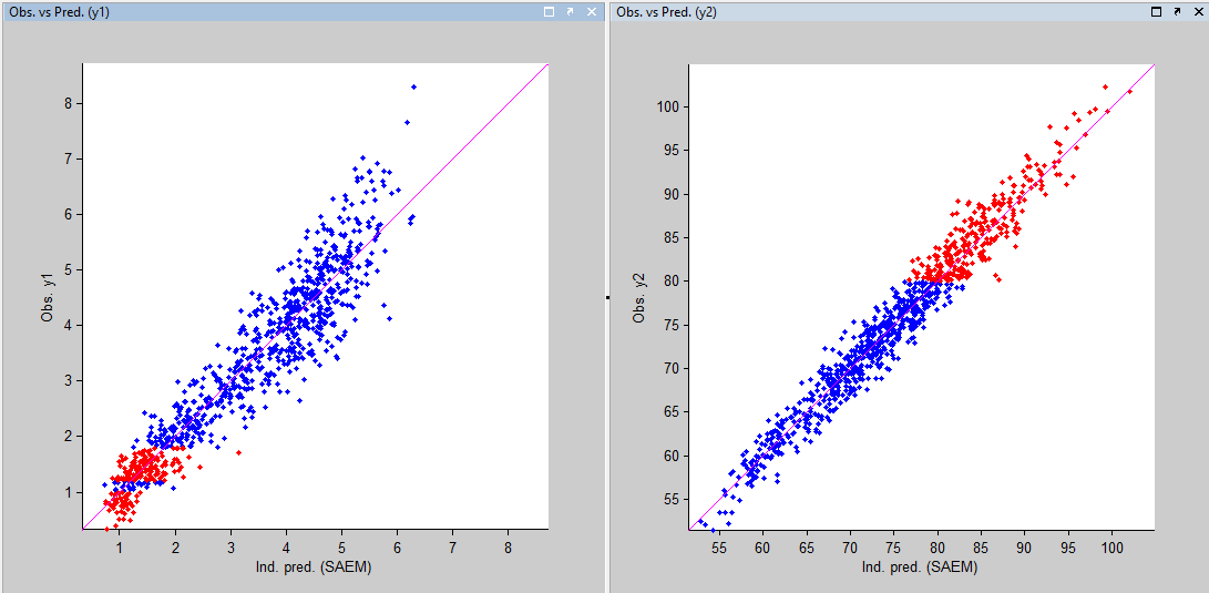
Other diagnostic plots, such as the plot of observations versus predictions, adequately use imputed censored PK and PD data:
Case studies
- 8.case_studies/hiv_project (data = ‘hiv_data.txt’, model = ‘hivLatent_model.txt’)
- 8.case_studies/hcv_project (data = ‘hcv_data.txt’, model = ‘hcvNeumann98_model_latent.txt’)