- Introduction
- Ordered categorical data
- Ordered categorical data with regression variables
- Discrete-time Markov chain
- Continuous-time Markov chain
Objectives: learn how to implement a model for categorical data, assuming either independence or a Markovian dependence between observations.
Projects: categorical1_project, categorical2_project, markov0_project, markov1a_project, markov1b_project, markov1c_project, markov2_project, markov3a_project, markov3b_project
Introduction
Assume now that the observed data takes its values in a fixed and finite set of nominal categories 
")

")


")


![\mathbb{P}(y_{ij}=c_k | \psi_i) \in [0,1]](http://s0.wp.com/latex.php?latex=%5Cmathbb%7BP%7D%28y_%7Bij%7D%3Dc_k+%7C+%5Cpsi_i%29+%5Cin+%5B0%2C1%5D&bg=ffffff&fg=000&s=0 "\mathbb{P}(y_{ij}=c_k | \psi_i) \in [0,1]")
 =1")


We can think, for instance, of levels of pain (low ")

")

 \leq \mathbb{P}(y_{ij} \preceq c_2 | \psi_i)\leq \ldots \leq \mathbb{P}(y_{ij} \preceq c_K | \psi_i) =1 .")
It is possible to introduce dependence between observations from the same individual by assuming that ")


 = \mathbb{P}(y_{ij} = c_k | y_{i,j-1},\psi_i).")
Ordered categorical data
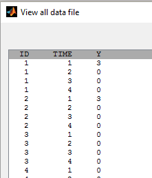
- categorical1_project (data = ‘categorical1_data.txt’, model = ‘categorical1_model.txt’)
In this example, observations are ordinal data that take their values in {0, 1, 2, 3}:
- Cumulative odds ratio are used in this example to define the model
)= \log \left( \frac{\mathbb{P}(y_{ij} \leq k)}{1 - \mathbb{P}(y_{ij} \leq k )} \right)")
where
) &=& \theta_{i,1}\\\text{logit}(\mathbb{P}(y_{ij} \leq 1)) &=& \theta_{i,1}+\theta_{i,2}\\\text{logit}(\mathbb{P}(y_{ij} \leq 2)) &=& \theta_{i,1}+\theta_{i,2}+\theta_{i,3}\\\end{array}")
This model is implemented in categorical1_model.txt:
[LONGITUDINAL]
input = {th1, th2, th3}
EQUATION:
lgp0 = th1
lgp1 = lgp0 + th2
lgp2 = lgp1 + th3
DEFINITION:
level = { type = categorical,  categories = {0, 1, 2, 3},
  logit(P(level<=0)) = th1
  logit(P(level<=1)) = th1 + th2
  logit(P(level<=2)) = th1 + th2 + th3
}
A normal distribution is used for 


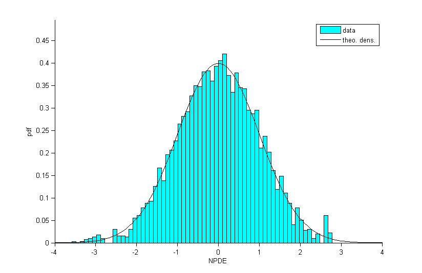
Residuals for noncontinuous data reduce to NPDE’s. We can compare the empirical distribution of the NPDE’s with the distribution of a standardized normal distribution:
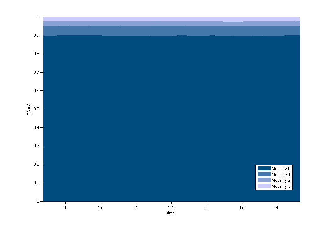
VPC’s for categorical data compare the observed and predicted frequencies of each category over time:

The prediction distribution can also be computed by Monte-Carlo:
Ordered categorical data with regression variables
- categorical2_project (data = ‘categorical2_data.txt’, model = ‘categorical2_model.txt’)
A proportional odds model is used in this example, where PERIOD and DOSE are used as regression variables (i.e. time-varying covariates)
Discrete-time Markov chain
If observation times are regularly spaced (constant length of time between successive observations), we can consider the observations
- markov0_project (data = ‘markov1a_data.txt’, model = ‘markov0_model.txt’)
In this project, states are assumed to be independent and identically distributed:
 = 1 - \mathbb{P}(y_{ij} = 2) = p_{i,1}")
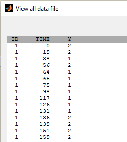
Observations in markov1a_data.txt take their values in {1, 2}. Before fitting any model to this data, it is possible to display the empirical transitions between states by selecting Transition probabilities in the list of selected plots.
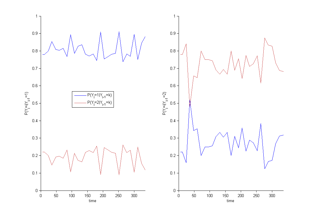
We can see that the probability to be in state 1 or 2 clearly depends on the previous state. The proposed model should therefore be discarted.
- markov1a_project (data = ‘markov1a_data.txt’, model = ‘markov1a_model.txt’)
Here,
 = 1 - \mathbb{P}(y_{i,j} = 2 | y_{i,j-1} = 1) = p_{i,11} \\\mathbb{P}(y_{i,j} = 1 | y_{i,j-1} = 2) = 1 - \mathbb{P}(y_{i,j} = 2 | y_{i,j-1} = 2) = p_{i,12} \\\end{aligned}")
[LONGITUDINAL]
input = {p11, p21}
DEFINITION:
State = {type = categorical,  categories = {1,2},  dependence = Markov
  P(State=1|State_p=1) = p11
  P(State=1|State_p=2) = p21
}
The distribution of the initial state is not defined in the model, which means that, by default,
 = \mathbb{P}(y_{i,1} = 2) = 0.5")
- markov1b_project (data = ‘markov1b_data.txt’, model = ‘markov1b_model.txt’)
The distribution of the initial state, ")
DEFINITION:
State = {type = categorical,  categories = {1,2},  dependence = Markov
  P(State_1=1)= p
  P(State=1|State_p=1) = p11
  P(State=1|State_p=2) = p21
}
- markov3a_project (data = ‘markov3a_data.txt’, model = ‘markov3a_model.txt’)
Transition probabilities change with time in this example:
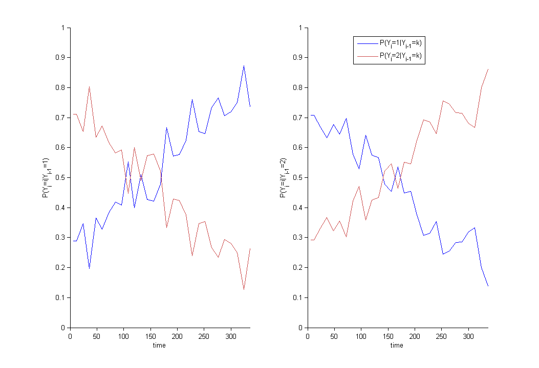
We then define time varying transition probabilities in the model:
[LONGITUDINAL]
input = {a1, b1, a2, b2}
EQUATION:
lp11 = a1 + b1*t/100
lp21 = a2 + b2*t/100
DEFINITION:
State = { type = categorical,  categories = {1,2},  dependence = Markov
  logit(P(State=1|State_p=1)) = lp11
  logit(P(State=1|State_p=2)) = lp21
}
- markov2_project (data = ‘markov2_data.txt’, model = ‘markov2_model.txt’)
Observations in markov2_data.txt take their values in {1, 2, 3}. Then, 6 transition probabilities need to be defined in the model.
Continuous-time Markov chain
The previous situation can be extended to the case where time intervals between observations are irregular by modeling the sequence of states as a continuous-time Markov process. The difference is that rather than transitioning to a new (possibly the same) state at each time step, the system remains in the current state for some random amount of time before transitioning. This process is now characterized by transition rates instead of transition probabilities:
 = k\,|\,y_{i}(t)=\ell , \psi_i) = h \, \rho_{\ell k}(t,\psi_i) + o(h),\qquad k \neq \ell .")
The probability that no transition happens between 

 = \ell, \forall s\in(t, t+h) \ | \ y_{i}(t)=\ell , \psi_i) = e^{h \, \rho_{\ell \ell}(t,\psi_i)} .")
Furthermore, for any individual )")

 = 0.")
Constructing a model therefore means defining parametric functions of time ")
- markov1c_project (data = ‘markov1c_data.txt’, model = ‘markov1c_model.txt’)
Observation times are irregular in this example:
Then, a continuous time Markov chain should be used in order to take into account the Markovian dependence of the data:
DEFINITION:
State = { type = categorical,  categories = {1,2}, dependence = Markov
  transitionRate(1,2) = q12
  transitionRate(2,1) = q21
}
- markov3b_project (data = ‘markov3b_data.txt’, model = ‘markov3b_model.txt’)
Time varying transition rates are used in this example.