- Introduction
- Computing the Maximum a posteriori (MAP) estimate
- Estimating the posterior distribution
- Fixing the value of a parameter
- Bayesian estimation of several population parameters
Objectives: learn how to combine maximum likelihood estimation and Bayesian estimation of the population parameters.
Projects: theobayes1_project, theobayes2_project, theobayes3_project
Introduction
The Bayesian approach considers the vector of population parameters 

 &= \frac{\pi_\theta( \theta )p(y | \theta )}{p(y)} \\ &= \frac{\pi_\theta( \theta ) \int p(y,\psi |\theta) \, d \psi}{p(y)} . \end{aligned}")
We can estimate this conditional distribution and derive statistics (posterior mean, standard deviation, quantiles, etc.) and the so-called maximum a posteriori (MAP) estimate of
 \\ &=\text{arg~max}_{\theta} \left\{ {\cal LL}_y(\theta) + \log( \pi_\theta( \theta ) ) \right\} . \end{aligned}")
The MAP estimate maximizes a penalized version of the observed likelihood. In other words, MAP estimation is the same as penalized maximum likelihood estimation. Suppose for instance that 

 + \frac{1}{\gamma^2}(\theta - \theta_0)^2 \right\} .")
This is a trade-off between the MLE which minimizes the deviance, ")
^2")

All things considered, the problem comes down to knowing whether the data contains sufficient information to answer a given question, and whether some other information may be available to help answer it. This is the essence of the art of modeling: find the right compromise between the confidence we have in the data and our prior knowledge of the problem. Each problem is different and requires a specific approach. For instance, if all the patients in a clinical trial have essentially the same weight, it is pointless to estimate a relationship between weight and the model’s PK parameters using the trial data. A modeler would be better served trying to use prior information based on physiological knowledge rather than just some statistical criterion.
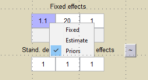
Generally speaking, if prior information is available it should be used, on the condition of course that it is relevant. For continuous data for example, what does putting a prior on the residual error model’s parameters mean in reality? A reasoned statistical approach consists of including prior information only for certain parameters (those for which we have real prior information) and having confidence in the data for the others. Monolix allows this hybrid approach which reconciles the Bayesian and frequentist approaches. A given parameter can be
- a fixed constant if we have absolute confidence in its value or the data does not allow it to be estimated, essentially due to lack of identifiability.
- estimated by maximum likelihood, either because we have great confidence in the data or no information on the parameter.
- estimated by introducing a prior and calculating the MAP estimate or estimating the posterior distribution.
Computing the Maximum a posteriori (MAP) estimate
- theobayes1_project (data = ‘theophylline_amt_data.txt’ , model = ‘lib:oral1_1cpt_kaVCl.txt’)
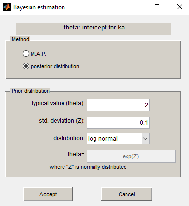
We want to introduce a prior distribution for 
Prior
We propose to use a log-normal distribution with mean ")

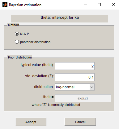
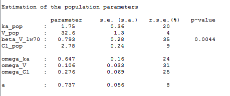
The MAP estimate of
Estimating the posterior distribution
- theobayes2_project (data = ‘theophylline_amt_data.txt’ , model = ‘lib:oral1_1cpt_kaVCl.txt’)
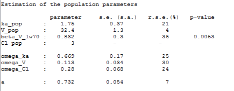
Using the same prior distribution, we can choose to estimate the posterior distribution of
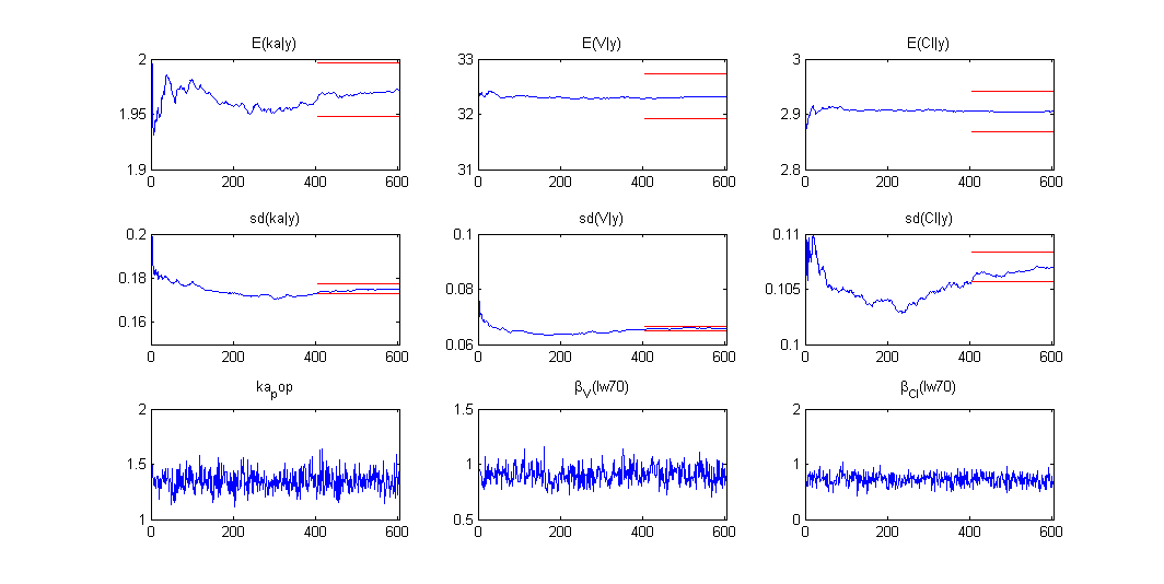
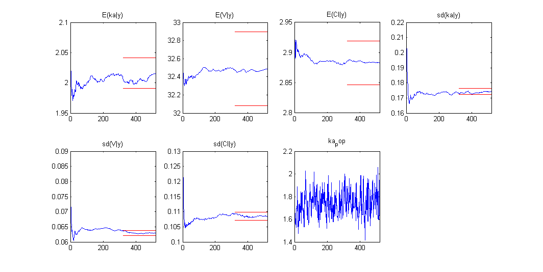
Estimation of the individual parameters using the conditional mean and sd is checked in this example. Then, the MCMC algorithm used for estimating the conditional distributions of the individual parameters is also used for estimating the posterior distribution of
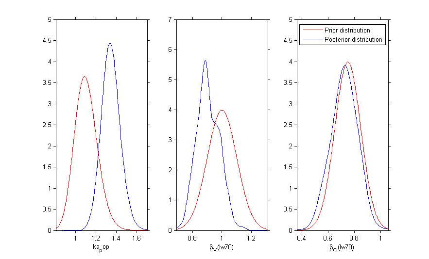
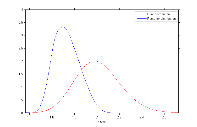
Once the (population and individual) parameters have been estimated, the posterior and prior distributions of
Fixing the value of a parameter
- theobayes3_project (data = ‘theophylline_amt_data.txt’ , model = ‘lib:oral1_1cpt_kaVCl.txt’)
We can combine different strategies for the population parameters: Bayesian estimation for 

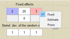
Remark: 
Bayesian estimation of several population parameters
- theobayes4_project (data = ‘theophylline_amt_data.txt’ , model = ‘lib:oral1_1cpt_kaVCl.txt’)
Prior distributions can be used for several parameters:
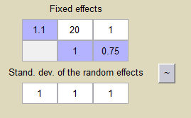
Then, the MCMC algorithm is used for estimating these 3 posterior distributions: