Inter occasion variability (IOV)

Introduction
Cross over study
Occasions with washout
Occasions without washout
Multiple levels of occasions

Objectives: learn how to take into account inter occasion variability (IOV).

Projects: iov1_project, iov2_project, iov3_project, iov4_project

Introduction

A simple model consists of splitting the study into K time periods or occasions and assuming that individual parameters can vary from occasion to occasion but remain constant within occasions. Then, we can try to explain part of the intra-individual variability of the individual parameters by piecewise-constant covariates, i.e., occasion-dependent or occasion-varying (varying from occasion to occasion and constant within an occasion) ones. The remaining part must then be described by random effects. We will need some additional notation for describing this new statistical model. Let

$\psi_{ik}$ be the vector of individual parameters of individual i for occasion k, where $1\leq i \leq N$ and $1\leq k \leq K$ .
${c}_{ik}$ be the vector of covariates of individual i for occasion k. Some of these covariates remain constant (gender, group treatment, ethnicity, etc.) and others can vary (weight, treatment, etc.).

Let $\psi_i = (\psi_{i1}, \psi_{i2}, \ldots , \psi_{iK})$ be the sequence of K individual parameters for individual i. We also need to define:

$\eta_i^{(0)}$ , the vector of random effects which describes the random inter-individual variability of the individual parameters,
$\eta_{ik}^{(1)}$ , the vector of random effects which describes the random intra-individual variability of the individual parameters in occasion k, for each $1\leq k \leq K$ .

Here and in the following, the superscript (0) is used to represent inter-individual variability, i.e., variability at the individual level, while superscript (1) represents inter-occasion variability, i.e., variability at the occasion level for each individual. The model now combines these two sequences of random effects:

$h(\psi_{ik}) = h(\psi_{\rm pop})+ \beta(c_{ik} - c_{\rm pop}) + \eta_i^{(0)} + \eta_{ik}^{(1)} .$

Remark: Individuals do not need to share the same sequence of occasions: the number of occasions and the times defining the occasions can differ from one individual to another.

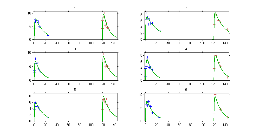
Cross over study

iov1_project (data = ‘iov1_data.txt’, model = ‘lib:oral1_1cpt_kaVk.txt’)

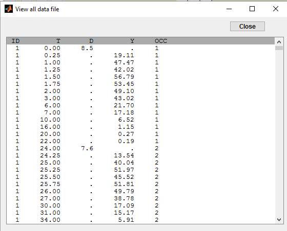
In this example, PK data are collected for each patient during two independent treatment periods of time (each one starting at time 0). A column OCC is used to identify the period:

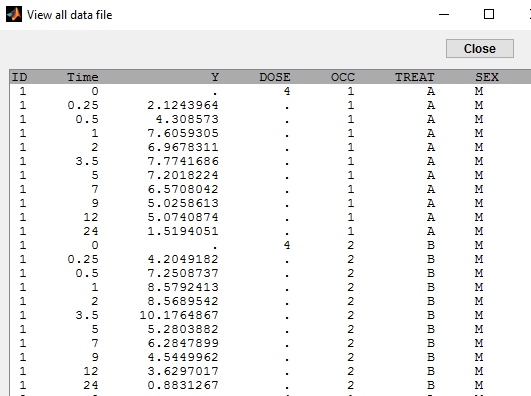
This column is defined using the reserved keyword OCC:

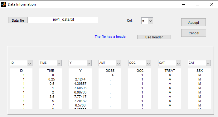
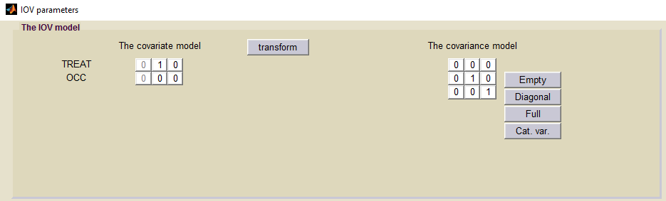
Here, treatment (column TREAT) changes with the occasion. Then, Monolix automatically creates a categorical covariate sTREAT which is the sequence of treatments (AB or BA). This new categorical covariates doesn’t change with time and can be used at the individual level” with SEX. We first define the distribution of the individual parameters at the “individual level” as usual:

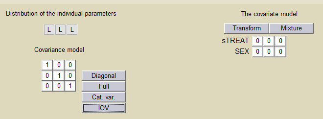
By clicking on the button IOV, we then define the distribution of the individual parameters at the occasion level”. In this example, we assume that the volume $V_i$ depends on the treatment we assume inter-occasion variability for $V_i$ and $Cl_i$ :

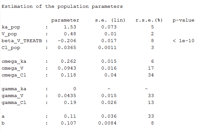
The population parameters now include the standard deviations of the random effects for the 2 levels of variability (omega is used fo IIV and gamma for IOV):

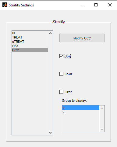
By clicking on Stratify in the menu bar of the graphics, you can use the occasion to split the plots

VPC per occasion:

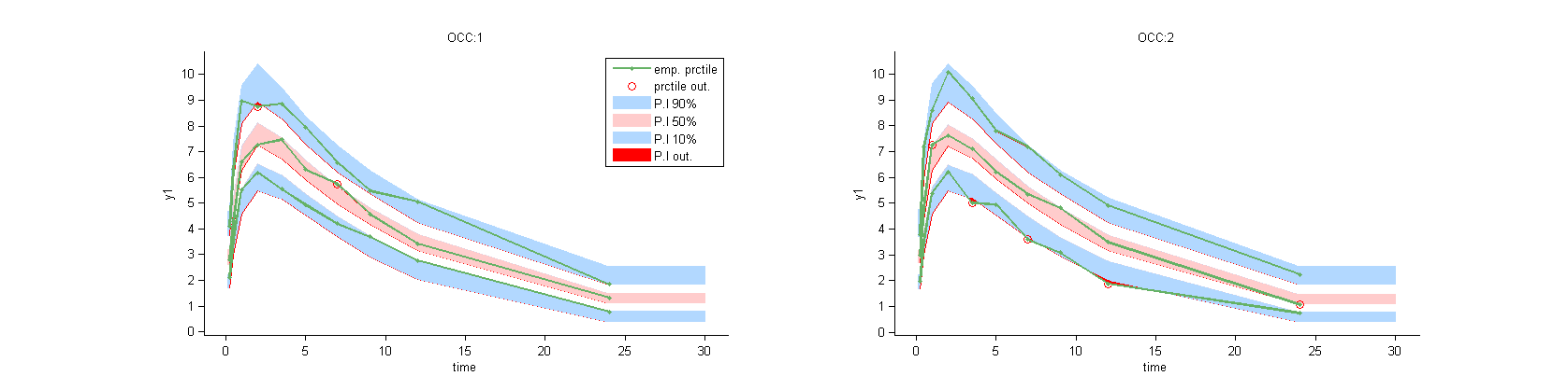
Prediction distribution per plot:

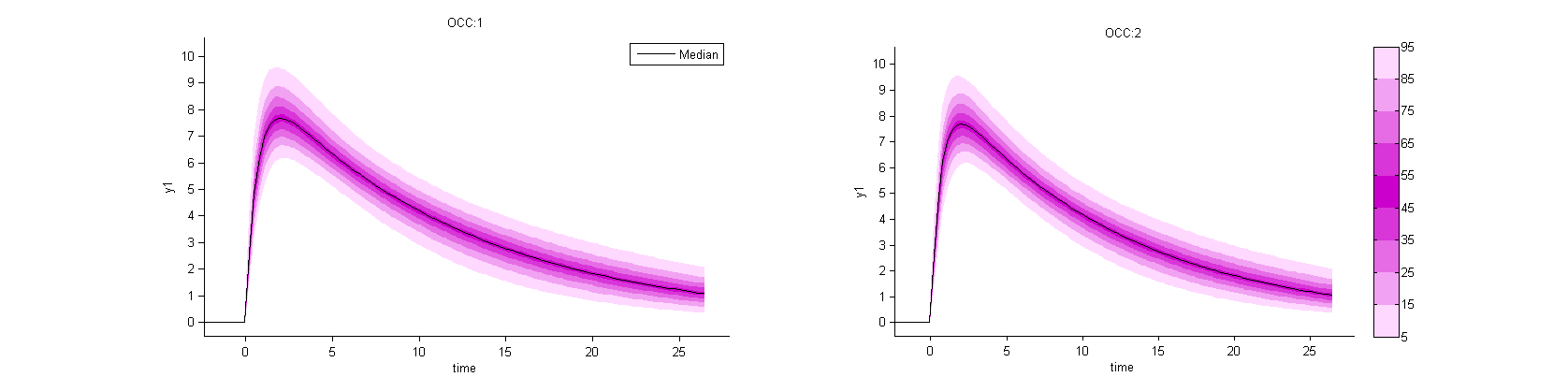
Occasions with washout

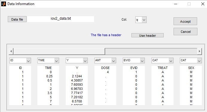
iov2_project (data = ‘iov2_data.txt’, model = ‘lib:oral1_1cpt_kaVk.txt’)

The time is increasing in this example, but the dynamical system (i.e. the compartments) is reset when the second period starts. Column EVID provides some information about events concerning dose administration. In particular, EVID=4 indicates that the system is reset (washout) when a new dose is administrated

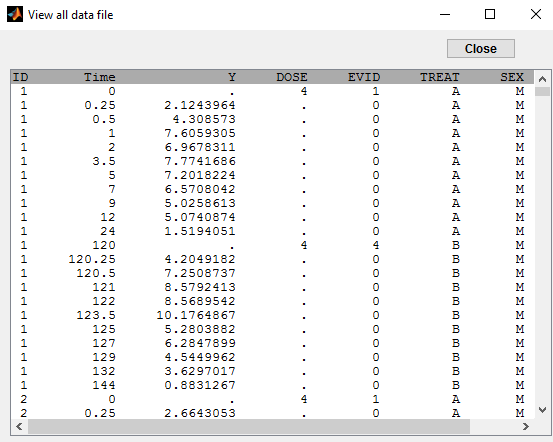
This column is defined using the reserved keyword EVID:

Monolix automatically proposes to define the treatment periods (between successive resetting) as statistical occasions and introduce IOV, as we did in the previous example. We can display the individual fit by splitting each occasion for each individual

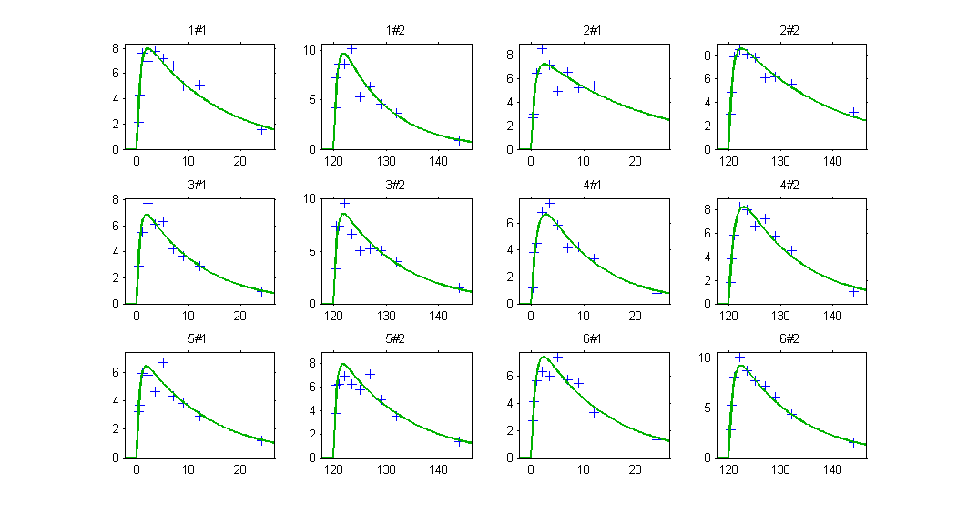
Or by merging the different occasions in a unique plot for each individual:

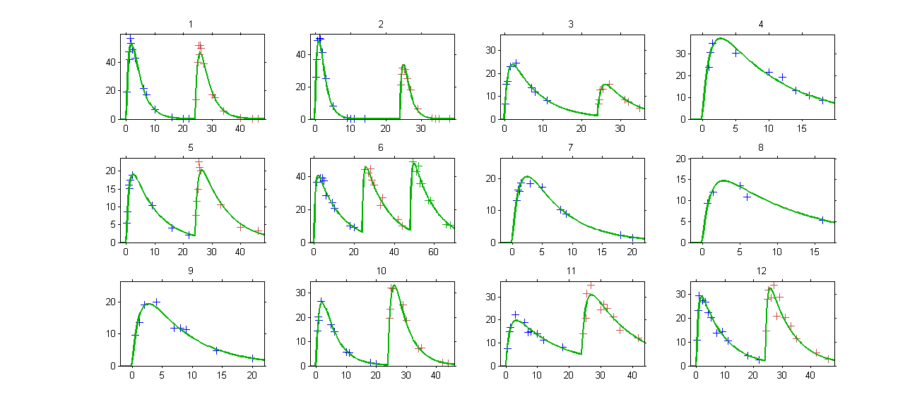
Occasions without washout

iov3_project (data = ‘iov3_data.txt’, model = ‘lib:oral1_1cpt_kaVk.txt’)

Multiple doses are administrated to each patient. We consider each period of time between successive doses as an statistical occasion. A column OCC is therefore necessary in the data file:

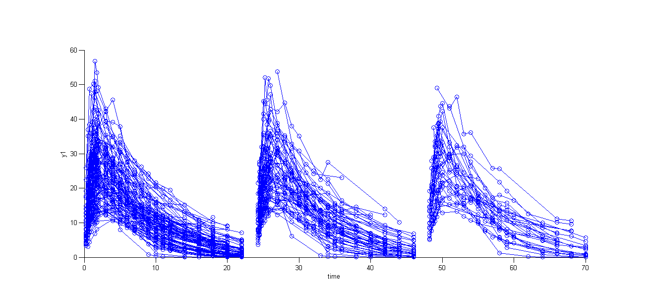
The model for IIV and IOV can then be defined as usual. The plot of individual fits allows us to check that the predicted concentration is now continuous over the different occasions for each individual:

Multiple levels of occasions

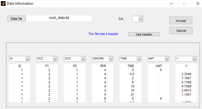
iov4_project (data = ‘iov4_data.txt’, model = ‘lib:oral1_1cpt_kaVk.txt’)

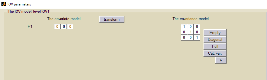
We can easily extend such approach to multiple levels of variability. In this example, columns P1 and P2 define embedded occasions. The are both defined as occasions:

We then define a statistical model for each level of variability. We can switch to the next/previous level by clicking on the arrow button